How much for my car? Using machine learning to find out

Intro

I own a wonderful Ford Fiesta ST-3 (2017, 7th generation, 38k miles), but since moving to London, she’s been sat at my parents’ house. I finally accepted it’s best to sell her. But how much should I ask?

Let’s do some data analysis and machine learning!

The JupyterLab notebook, extractor script, and data, is available on Github: https://github.com/jamesdeluk/data-science/tree/main/Projects/car-price-regression-modelling

Gather the data

Auto Trader makes it difficult to scrape data - the page is loaded dynamically, and has robots.txt etc to restrict bots, so I couldn’t find an online tool that worked. They do provide an API, but that’s only for industry, and likely costs a pretty penny.

I could create a Selenium script; however, as I only need to get the data once, I decided for a quicker, albeit more manual option - sometimes more tech is not the solution.

First, filter for the cars I want to scrape. There’s no way to include ST-2s and ST-3s, so I had to use two filters:

https://www.autotrader.co.uk/car-search?make=Ford&model=Fiesta&aggregatedTrim=ST-3&exclude-writeoff-categories=on

https://www.autotrader.co.uk/car-search?make=Ford&model=Fiesta&aggregatedTrim=ST-2&exclude-writeoff-categories=on

Second, create a Stylus style to hide/remove a lot of the unneeded DOM elements:

section.atds-header-wrapper, main#content article div.at__sc-1okmyrd-3, div.at__sc-1iwoe3s-7, li:last-of-type, #footer-container, figure, .at__sc-1iwoe3s-3 {
    display: none;
}

Third, manually copy and paste each page to a text file. There are ~640 cars in total, so ~64 pages; it took a while, but not too long.

Fourth, I asked an LLM to write a script to extract the data I wanted - Price, Year, Mileage, Distance (from me / the location of the car), Trim, Generation, and Seller type. The first attempt wasn’t perfect, but with several more prompts and some manual tweaking, it worked:

import re
import csv

## Function to clean text by removing lines with invalid £ symbols
def clean_text(text):
    # Define a valid price pattern
    valid_price_pattern = r'^£\d{1,3}(?:,\d{3})*$'  # Matches only full price lines like £9,999
    
    cleaned_lines = []
    for line in text.splitlines():
        # If the line has a £ symbol, keep it only if it matches the valid price pattern
        if '£' in line:
            if re.match(valid_price_pattern, line.strip()):
                cleaned_lines.append(line)
        else:
            # Keep lines without £ symbols
            cleaned_lines.append(line)
    
    return "\n".join(cleaned_lines)

## Function to extract data
def extract_data(text):
    # Define regex patterns
    price_pattern = r'£(\d{1,3}(?:,\d{3})*)'  # Matches price like £9,999
    year_pattern = r'(\d{4})(?: \(\d+ reg\))?'  # Matches year with or without (reg)
    mileage_pattern = r'(\d{1,3}(?:,\d{3})*) miles'  # Matches mileage like 38,032 miles
    engine_pattern = r'(1\.\d)'  # Matches engine size like 1.5L or 1.6L
    distance_pattern = r'\((\d+) miles\)'  # Matches distance like (1 miles)
    seller_pattern = r'reviews|See all \d+ cars'  # Matches reviews and "See all cars" for seller type
    trim_pattern = r'ST-\d'  # Matches ST trim level like ST-2, ST-3

    # Define generation based on engine size
    generation_mapping = {'1.6': 7, '1.5': 8}

    data = []
    
    # Split the text into chunks starting with a price (£)
    entries = re.split(r'(£\d{1,3}(?:,\d{3})*)', text)  # Splitting with prices included
    for i in range(1, len(entries), 2):  # Process every second entry (price and car details)
        price = entries[i].replace('£', '').replace(',', '')  # Clean price
        chunk = entries[i+1]
        
        # Extract other fields
        year_match = re.search(year_pattern, chunk)
        mileage_match = re.search(mileage_pattern, chunk)
        engine_match = re.search(engine_pattern, chunk)
        distance_match = re.search(distance_pattern, chunk)
        seller_match = re.search(seller_pattern, chunk)
        trim_match = re.search(trim_pattern, chunk)  # Extract trim level
        
        # Extract fields
        year = year_match.group(1) if year_match else ''
        mileage = mileage_match.group(1).replace(',', '') if mileage_match else ''
        engine_size = engine_match.group(1) if engine_match else ''
        generation = generation_mapping.get(engine_size, '')
        distance = distance_match.group(1) if distance_match else ''
        seller = "Trade" if seller_match else "Private"  # "trade" for dealer, "private" for private seller
        trim_level = trim_match.group(0) if trim_match else ''  # Extract trim level (ST-2, ST-3)

        # Check for empty fields
        if not price or not year or not mileage or not generation or not distance:
            print(f"Alert: Incomplete entry found: Price: {price}, Year: {year}, Generation: {generation}, Trim: {trim_level}, Mileage: {mileage}, Distance: {distance}, Seller: {seller}")

        # Append the extracted data as a row
        data.append([price, year, generation, trim_level, mileage, distance, seller])
    
    return data

## Read the text file
input_file = 'raw_car_data.txt'
with open(input_file, 'r', encoding='utf-8') as file:  # Added encoding='utf-8'
    raw_text = file.read()

## Clean the text to remove invalid £ lines
cleaned_text = clean_text(raw_text)

## Extract data
car_data = extract_data(cleaned_text)

## Write to a CSV file
output_file = 'car_data.csv'
with open(output_file, 'w', newline='', encoding='utf-8') as csvfile:  # Ensure writing in UTF-8 too
    writer = csv.writer(csvfile)
    # Write header
    writer.writerow(['Price', 'Year', 'Generation', 'Trim', 'Mileage', 'Distance', 'Seller'])
    # Write data
    writer.writerows(car_data)

print(f'Data extraction complete. CSV file saved as {output_file}')

I now had a .csv of >600 car data! Time to start processing.

One thing to note: This is the asking price on the website, not the actual selling price.

Cleaning the data

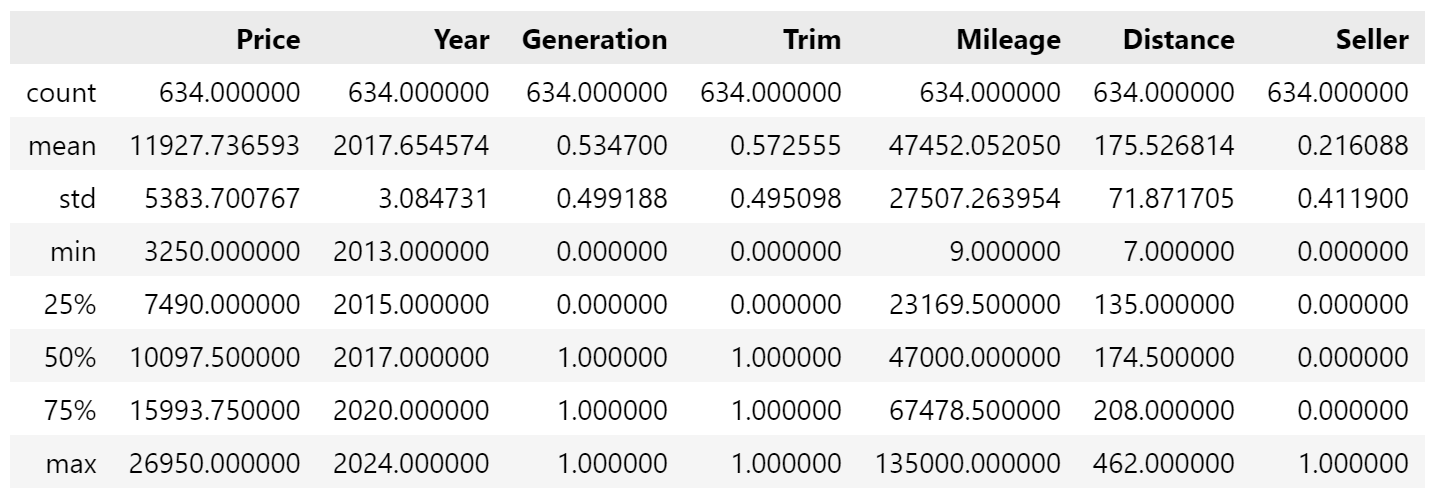
Now for quality control. Let’s see what we’ve got, starting with .head() and .describe():

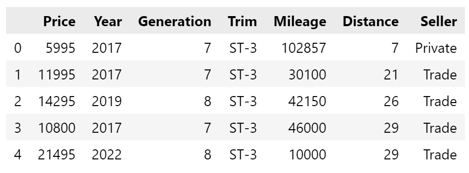
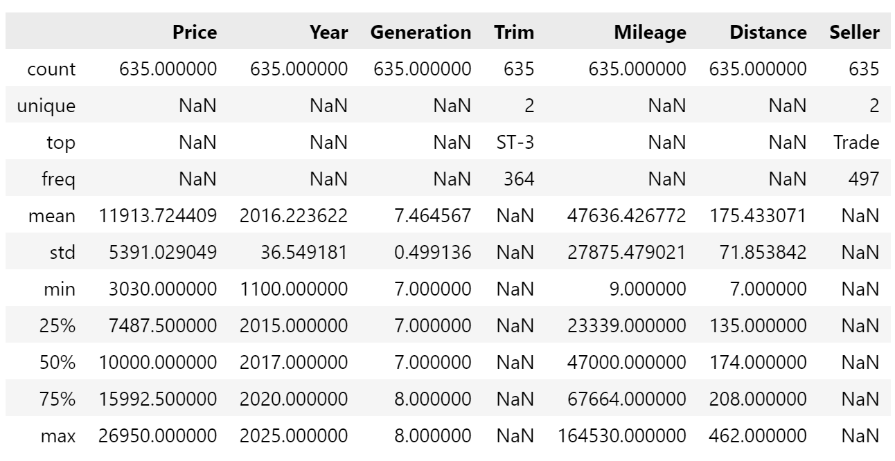
We have 635 cars in the dataset, ranging from ~£3000 to ~£27,000. The average car is a 2016 7th gen (as generation is an integer) with 47k miles and being located 175 miles from mine, with an asking price of just over £11,900. Trim and Seller has NaN (not a number) for the stats because they’re text values, although it does state Trade an ST-3s are most common.

Nulls

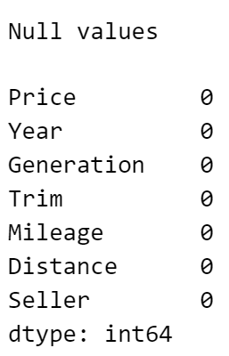
First, null/missing values, found using .isnull().sum(). If there were some, I would tweak the extraction script and re-check it had got all the data, until we got 0 for all:

Remapping

Second, I did some remapping of values. There were three columns with only two values, confirmed by .nunique(): Generation (7 or 8), Trim (ST-2 or ST-3), and Seller (Trade or Private). Analysis works better with binary values, so I remapped based on mine being 1s - that is, Generation 7 to 1 and 8 to 0, ST-3 to 1 and ST-2 to 0, and Private to 1 and Trade to 0.

Outliers

Third, outliers. .describe() and boxplots were useful.

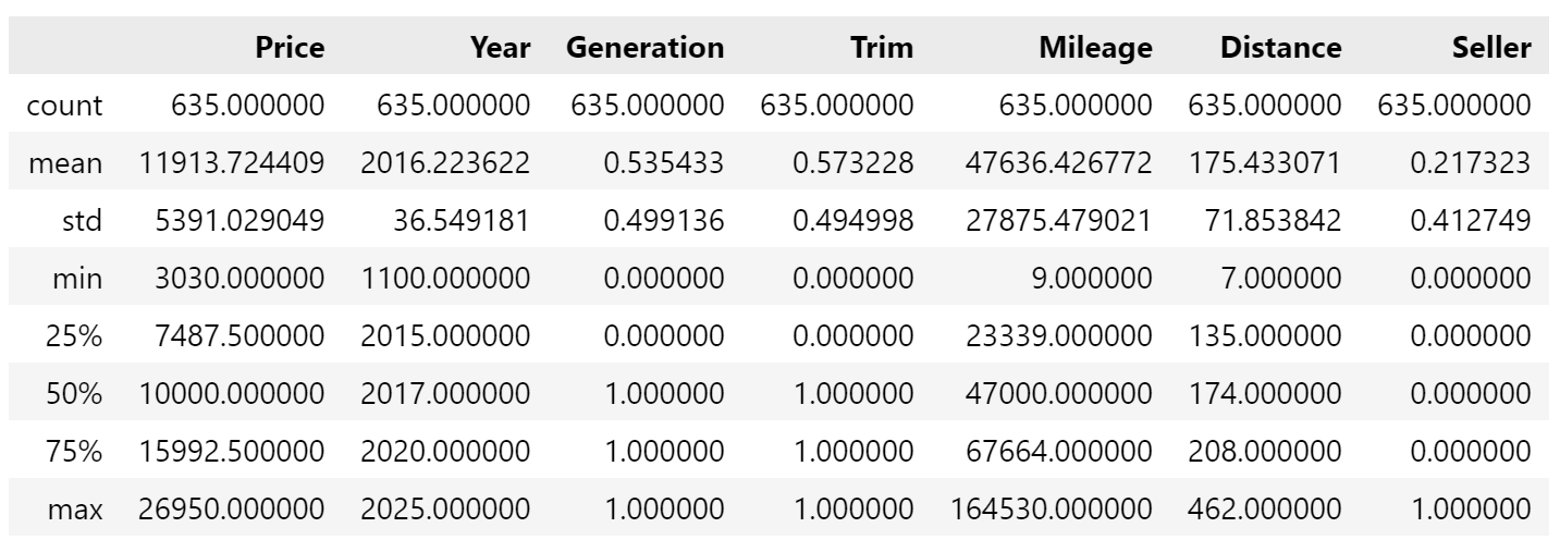
For example, the former gave the max Year as 2025 (which is in the future, so impossible), and the latter showed that the car with Mileage of 164,500 miles an outlier. Both showed one car with a Year of 1100, which also seemed unlikely.

I went back the original data to get the correct years, and simply removed the individual car with incredibly high mileage. There was one car with a Mileage of only 9, but checking the data, this seemed legit - it was a brand new car.

This looks better, although Distance has many points outside the interquartile range.

Splitting

Everything looks good, so finally I simply split the data into groups for future use. In particular, I made gen7_st3_private_data_dropped, which was (as the name suggests) only privately-sold 7th generation ST-3s (like mine), with the columns for Generation/Trim/Seller dropped (as they all contain the same values, so add nothing to analyses). In general, I will split the analysis into cars very similar to mine (the “alikes”), using this dataset, and for all cars, using the entire data dataset.

Exploratory data analysis

Now the data was ready, I wanted to briefly see how mine compared. .describe() was good for this. My car is younger slightly than average, and the Mileage is >20% less than the mean.

Scattering

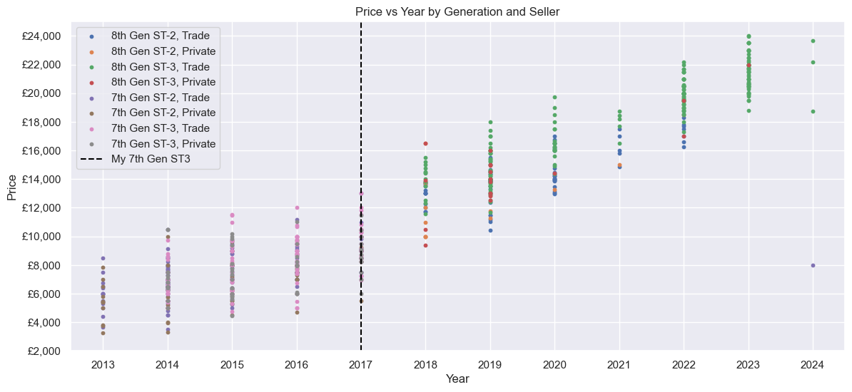
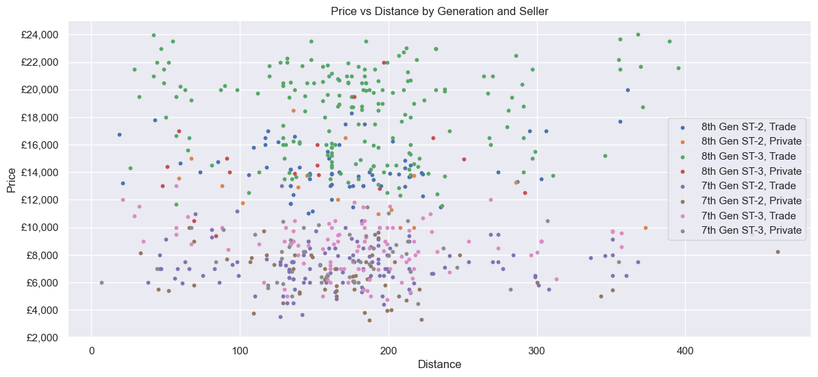
What does the data look like? Let’s plot all the data. There is a linear-ish relationship between Price and Mileage, but not perfectly so - mostly due to the two Generations. Price clearly goes up with Year. Distance seems to have no correlation, although they seemed to be bunched between ~130 and ~230 miles away.

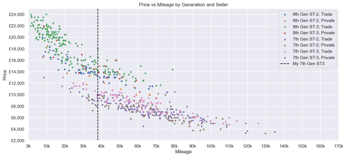
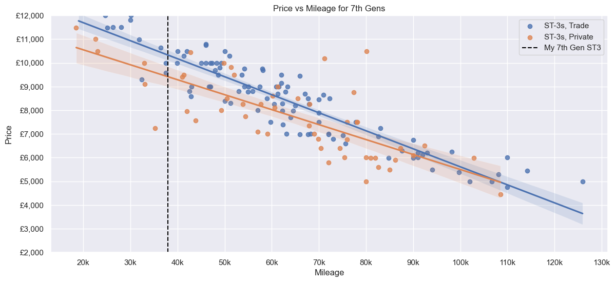
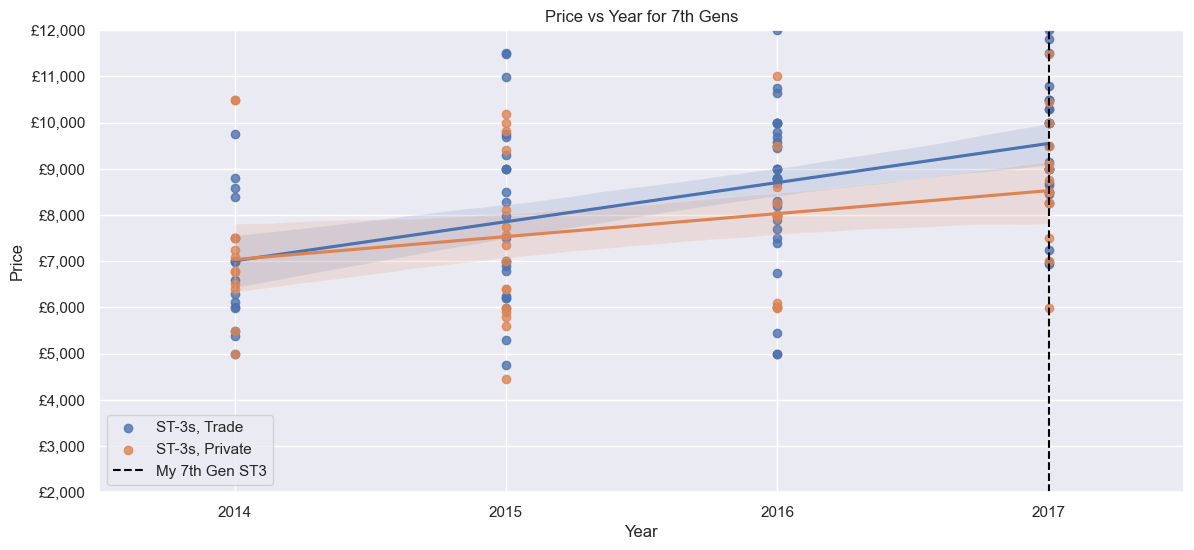
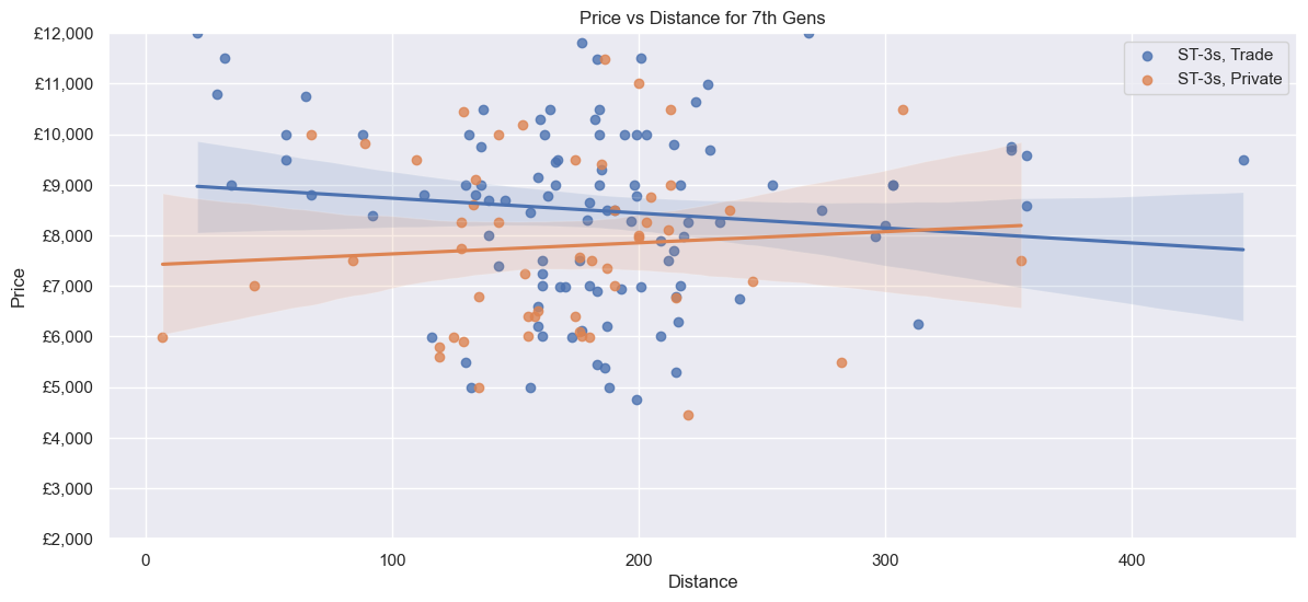
Next, only the 7th Gen ST-3s. The relationship between Price and Mileage in particular looks linear, although there are some outliers. A Private seller could ask ~£9000 to ~£9800 for a car with 38k Mileage, whereas a Trade seller could ask for ~£1000 more (albeit with a smaller range). Distance is similar to before - no correlation, most ~130 to ~230 miles away.

Histograms

Histograms are used to see the distribution of the data. If the data is normally distributed, linear regression is okay. If it is not, linear regression is no good.

Across all the data, only Distance is roughly normally distributed. For 7th Generation, Mileage and Price are also fairly normally distributed, but with some skew (positive for Price, negative for Mileage).

Q-Q plots

Q-Q (quantile–quantile) plots can also show if a linear regression is good. A straight line in the plot suggests a linear relationship. For all data, Price, Year, and Mileage are mostly S-shaped, so slightly linear, but not really. Again, the alikes appear to be more linear.

Scipy statistics

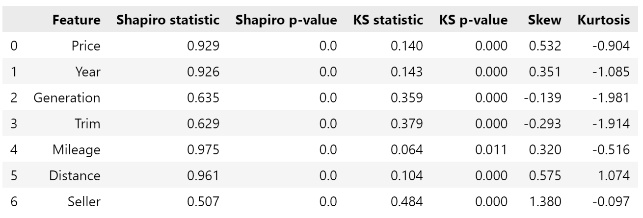
More linearity! This time with the scipy module, which can measure. Shapiro, Kolmogorov-Smirnov (KS), and skew/kurtosis. Firstly, for all data:

And then just for the alikes:

Shapiro statistics closer to 1 suggest higher linearity; several of the features, for both datasets, have statistics over 0.9, which suggests normality. However, a low p-value (say, <0.05) suggests they deviate from normality - in this case, all the features for all data, and Year for the alikes.

Unlike Shapiro, lower KS statistics suggest linearity, but like Shapiro, low p-values suggest deviation. Based on this, most all data features are not normal (except perhaps Mileage), and some alikes features may be normal-ish.

Based on both of these, Price, Mileage, and Distance for alikes may be normal-ish - a similar observation to the histograms and Q-Q plots (starting to see a pattern here eh?)

Skew relates to symmetry, and kurtosis relates to tails. A normal distribution is symmetrical (skew of 0), and kurtosis of 0 implies the tails follow the normal distribution. Much of the data has some skew, either positive or negative, although Year for alikes is pretty good, and the others alikes aren’t too bad. Low kurtosis values suggest few outliers, high kurtosis suggests many - Distance definitely has the most, with aligns with what we saw in the box plots.

Pandas correlations

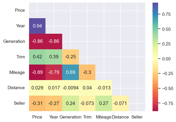
And finally, correlations. Pandas supports three types of correlation coefficients - Pearson, Kendall Tau, and Spearman’s rank. All showed similar results. For the full dataset, Price is strongly positively correlated with Year, and strongly negatively correlated with Generation (remember, 1 is the older model) and Mileage. Trim is mildly positive, Seller is mildly negative. Distance shows almost no correlation (as the scatters suggest also).

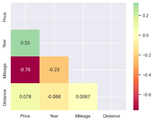
It’s similar for the alikes, simply with fewer features.

Multicollinearity

Multicollinearity measures how much one feature varies with another. Using variation inflation factor from statsmodels:

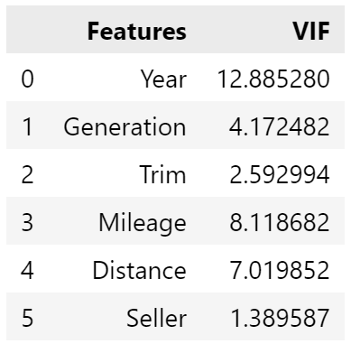
Typically, a value over 10, such as Year, is bad, and should be removed. However, I don’t like the idea of removing it - if I was considering buying a car, year is important. So, for now, I’ll leave it in.

Clustering

One more thing. This isn’t really an exercise where clustering would be helpful, but I wanted to see what showed up anyway.

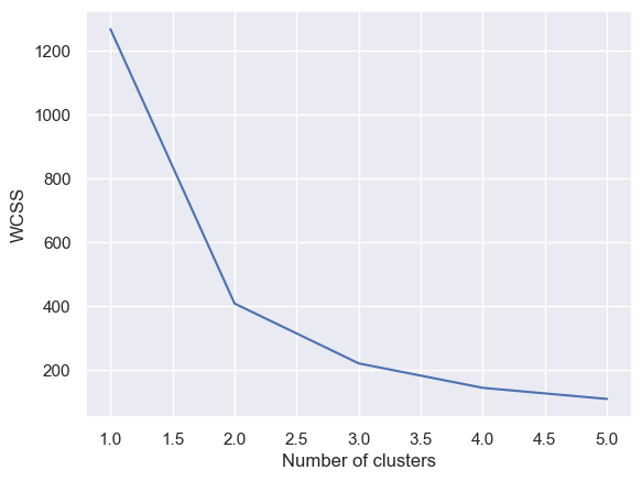
For Price vs Mileage for all data, the elbow is clearly at 2:

Giving a diagonal split:

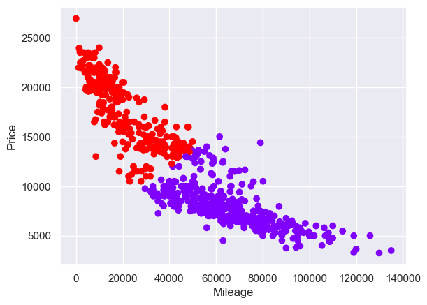
Not that we learn much from this.

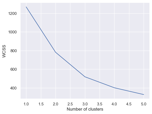
What about Price vs Distance? There was no clear elbow, but 3 looks slightly better:

Running the algorithm a few times mostly gave a split similar to the top one, but occasionally one more like the bottom:

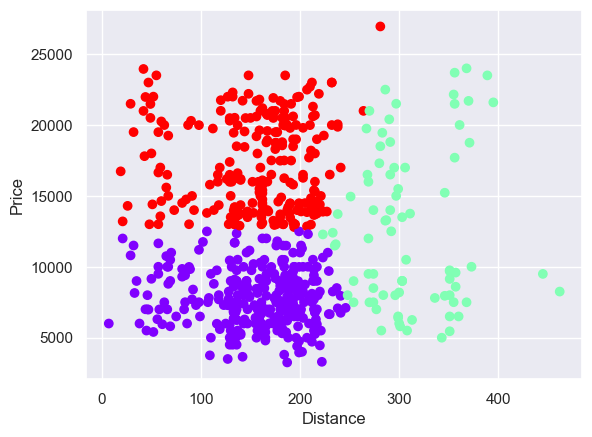
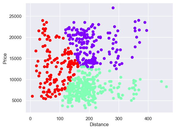
I was actually expecting a larger single cluster, given the density there.

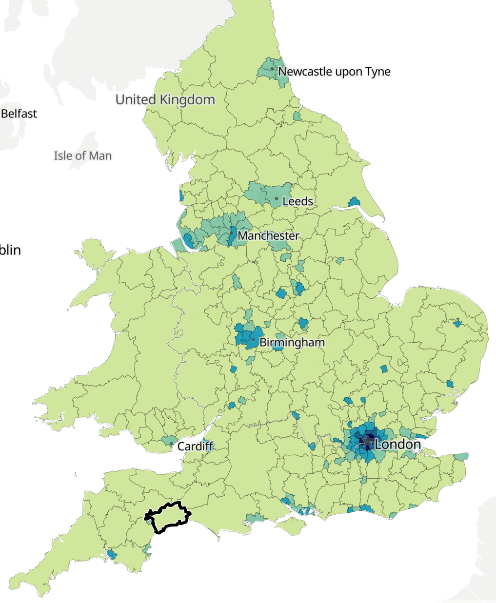
I thought it would be interesting to check this against a population map of the UK. Distance is measured from the black box in the map below (source: ONS), which is where the car is. The darker the colour, the higher the population density. London, Birmingham, and Manchester - the darker, high-density places - all fall in the 160-230 mile range, which correlates with the areas on scatter chart with many points.

Summary

Everything above suggests linear modelling might work for alikes, and for the full dataset, something more complex might be worthwhile. So I’ve decided to do two analyses, and compare them. Would they be similarly accurate? What about the predicted asking price?

Simple modelling for privately-sold generation 7 ST-3s

Statsmodels ordinary least squares

After getting the data ready, I did a simple linear regression - Ordinary Least Squares - using statsmodels. This is great, because alongside the coefficients, it provides P-values, R-squared values, F-statistics, and more.

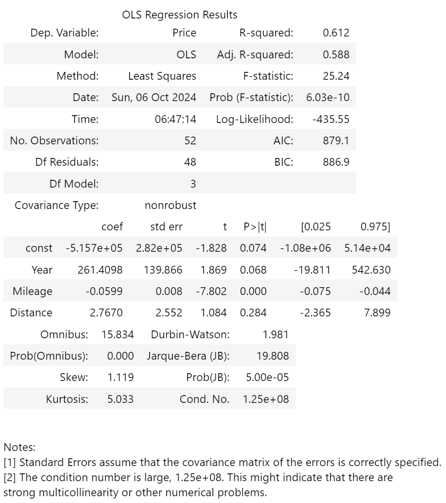
At this stage, the predicted price is £9262.

The R-squared suggests 61.2% of the variability is explained by the model, which is so-so. The adjusted R-squared is a bit lower, suggesting some features may not improve the model. The goal would be 100% for both, although this is near impossible.

The higher the F-statistic the better (typically >5 is good), and the lower the probability of it shows significance (typically <0.05 is good). This suggests the model is significant.

For log-likelihood, the closer the value is to zero the better. For the information criteria - Akaike, AIC, and Bayesian, BIC - the lower the better. These are best when comparing with other models.

Omnibus, skew, kurtosis, and Jarque-Bera measure normality. We’d want the middle two near 0, and the probabilities for omnibus and JB >0.05, for normality. This analysis suggests the features are not normal - even though previous analyses suggested they are relatively normal.

A Durbin-Watson value of 1.981 suggests no auto-correlation, which is good. The conditional number measures multicollinearity, which is something we don’t want. Over 30 - as this definitely is - suggests high multicollinearity (as the second note states, and we already knew from previous analyses).

A key observation at this time is that Distance has a P-value of 0.284. This is high - normally we’d want 0.05 or lower. A value this high suggests it doesn’t add much to our analysis (as we’d previously presumed from the graphs above). Also, the mean is 2.8, with a standard deviation of 2.6, giving a range of 0.2 to 5.4!

No Distance

So let’s remove it, and re-do the OLS:

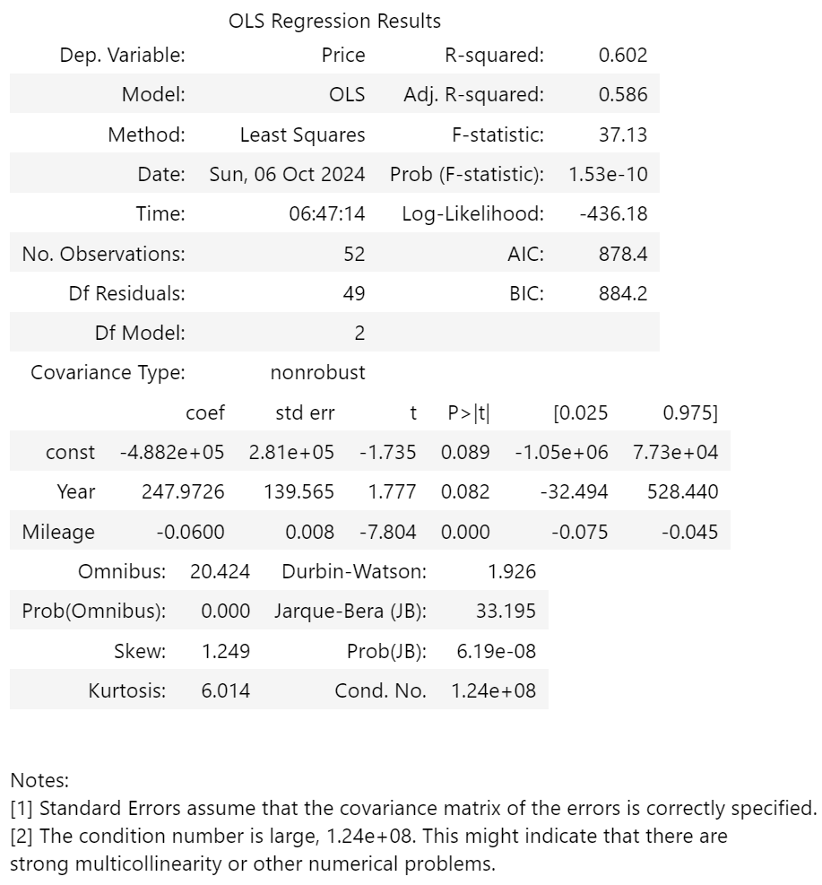
The adjusted R-squared drops minimally, suggesting it’s slightly less accurate (probably as we lost 1/3 of the features), but F-stat has improved, and it is still significant. LL, AIC, and BIC, barely changed, nor did the conditional number. The normality worsened slightly. Overall, the model didn’t particularly improve or deteriorate, but we have removed the statistically insignificant feature, which is good.

The predicted price jumps from £9262 to £9706. Given these coefficients, a year newer increases the price by £250, and every extra 1000 miles decreases the price by £60. The constant is heavily offset by the fact the years run from 2014 to 2017 - I reran the analysis with relative years (i.e. 2014 was 0, 2017 was 3), and whilst the coefficients and prediction stayed the same, the constant increased from -£488k to ~£11k.

Next I checked for variation inflation factors, to see how correlated the features are (i.e., if one goes up, will the other also go up). Ideally you want them disconnected, with a VIF of <5. However, we only have two, and both are 10.9 - not ideal. Normally you’d remove one, but I don’t want to drop to a single feature at this stage.

Sklearn linear regressions

Instead, we’ll try some other regressions. Using scikit-learn (sklearn) linear regressions - first, with unsplit data; then, with train_test_split data, using 10% of the data (so 5 test and 47 train); then cross-validated with 10 validations, assessing for best mean absolute error (MAE), mean squared error (MSE), and R² value (with the value printed the mean of all validations).

As expected, the results from the linear regression with sklearn were the same as with statsmodels - same method, different module.

The prediction with the split was £9563, so about 15% less than without the split. The simple MAE was 1160, which is high - over 10% of the final price. However, with cross-validating, this comes down to a mean of 857, which is still high, but at least <10%. The mean R² is terrible, -0.055, but not surprising given the small dataset and multicollinearity. And, when split, the Year coefficient drops by ~25%, and Mileage increases in magnitude by 3% - the split suggests Mileage is more important than previously thought, and Year less.

Lasso, ridge, elastic net regressions

There are other types of linear regressions, also part of sklearn, such as lasso, ridge, and elastic net. They take alpha values as a parameter. Similar to before, I cross-validated to find the best MAEs using default parameters, for a quick result, then I did a gridsearch to try other alpha values, to see if anything improves.

It turns out the lowest alpha was always the best (I kept testing lower and lower), and the results for all three models were the same. The best mean MAE improved by 10, to 847, with a mean R² of 0.6 (still not great, but getting there), and a prediction of £9618. Better, but marginally so.

Leave-one-out cross validation

Given the small dataset, I also thought I’d try leave-one-out cross validation, which uses a single datapoint for testing. The prediction was the same as the unsplit linear regression, £9706, but mean MAE was almost 3000!

No Distance no Year

Finally, I wanted to know what would happen if I also removed Year, given Year and Mileage were collinear, and some VIF testing suggested Year was the better one to remove. This would leave me with a single feature - in other words, Price vs Mileage - so I wasn’t hopeful I’d get a good result.

A quick OLS, and sklearn regressions:

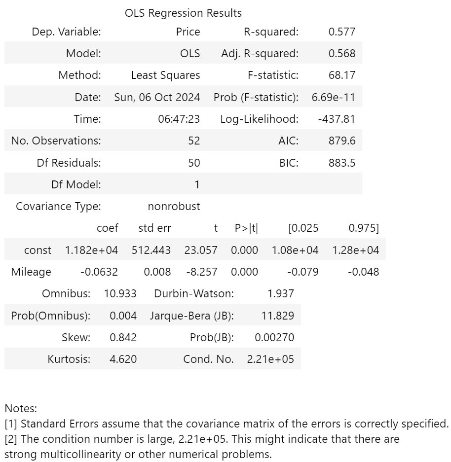
R² dropped slightly. F-stat improved. LL, AIC, BIC were all similar. The features were slightly more normal, and the conditional number dropped, but is still very high (even though there is only one feature?!) The coefficient, now that there is no Year, rises to ~£11k - the same we found when changing to relative years - and the gradient of the Mileage line increased by ~3%.

Predictions dropped to £9415 with unsplit data, £9313 with split data. Mean MAE was actually better, at 840, but the mean R² dropped to 0.089, which is terrible.

Rerunning the lasso/ridge/elastic net regressions returned a mean MAE of 871, and an R²of 0.577, so worse than with Year included.

Conclusion

The best turned out to be lasso with the Distance feature removed, with MAE of 847, R² of 0.602, and a prediction of £9618.

Standard linear regression with Year and Distance features removed had a fractionally lower MAE of 840, but an R² of <0.1, and a prediction of £9313.

More complex modelling using the entire dataset

Statsmodels ordinary least squares

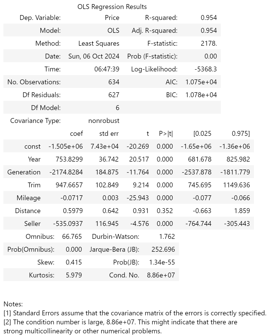
I again started with an OLS analysis; while I know the data isn’t linear, it would give insight into the different features. R-squared, F-stat are better, but LL/AIC/BIC significantly worse, than the alikes, due to the larger size of the dataset and the other features (which are all, apart from Distance, significant - although for now I’ll opt to keep Distance included). The data is still not normal, and there is still multicollinearity.

Quick predictions

First, I used a bunch of models (linear regression, decision tree regressor, random forest regressor, gradient boosting regressor, XGB regressor, all with default parameters and a fixed random_state), without splitting to data, to predict the prices. These varied from £9719 to £11,000, with a mean of £10,395 - significantly higher than the linear predictions based on the alikes.

Regressions with split data

Next I split the data, with train_test_split. This time I used 20% of the data, as we now have over 630 datapoints. Using the same models as above, the lowest mean absolute error (MAE) was 685 using gradient boosting, followed by 733 for random forest and 742 for XGBoost - all far better than the alikes modelling, at almost 850. R² were good too; these three were all above 0.970, compared with barely above 0.6 for alikes. Predictions were £9857, £10135, and £9917 respectively.

Cross-validation

Cross-validating (10 times) again has gradient boost as the best, this time with a slightly-lower MAE of 660, a standard deviation of 95, and a slightly worse (but still good) mean R² of 0.970. Random forest and XGBoost were again the next best; I’ll take all three to the next stage, hyperparameter tuning, to see how low I can get the MAE and how high the R².

Hyperparameter tuning: RandomizedSearchCV, GridSearchCV, BayesSearchCV

There are a few methods of hyperparameter tuning. RandomizedSearchCV allows you to assess a random selection of parameters from a grid; to demonstrate, I only did 10 iterations, but one of them with XGBoost gave an MAE of 626 and R² of 0.973 - the best so far. Predicted price of £9857 - yes, the same as gradient boosting above.

Total parameter combinations: 77,760

Best MAE: 626

Params: {‘subsample’: 0.7, ‘reg_lambda’: 0, ‘reg_alpha’: 0.5, ’n_estimators’: 500, ‘min_child_weight’: 3, ‘max_depth’: 3, ’learning_rate’: 0.01, ‘gamma’: 0.1, ‘colsample_bytree’: 0.8}

Mean R²: 0.973

Prediction: £9857

A more detailed tuning method is GridSearchCV, which tests every parameter combination in a grid. As you’d expect, this can take a long time. With the grids I chose, the total combinations were in the tens of thousands. I created a test in which I did 10 fits and timed it, then scaled it up. To complete the grid searches with my current hardware would take hours; for example, this was XGBoost:

Time taken for 10 fits: 2.8034 seconds

Total number of fits: 9000 x 15 = 135,000

Approximate time for all fits: 630.76 minutes

A third, more intelligent option, is BayesSearchCV. You provide a parameter grid with ranges for each parameter, and it uses Bayesian optimisation to find the best combination - the more iterations the better. I eventually did 200 iterations for each of the three models, as I found the time does not scale linearly - that is, 200 iterations took more than twice as long as 100. Also, in RandomizedSearchCV and GridSearchCV you provide the parameters, so they’re typically discrete; BayesSearchCV generates themselves, therefore you can get fun values - for example, I got a best learning rate 0.06218773088413575. Anyway, BayesSearchCV got my new best results. MAE of 614, R² of 0.973, and prediction of £10,096 for XGBoost, and MAE of 615, R² of 0.974, and prediction of £9499 for gradient boosting. Random forest was marginally worse, with an MAE of 648.

Best MAE: 614

Params: {‘colsample_bytree’: 0.7045595143703863, ‘gamma’: 0.27799738001688257, ’learning_rate’: 0.005295122282668858, ‘max_depth’: 3, ‘min_child_weight’: 6, ’n_estimators’: 1380, ‘reg_alpha’: 0.3602780543551241, ‘reg_lambda’: 0.0, ‘subsample’: 0.2771742081488788}

Number of interations: 200

R²: 0.97279

Prediction: £10096

Best MAE: 615

Params: {‘alpha’: 0.3156584410262337, ’learning_rate’: 0.06218773088413575, ‘max_depth’: 5, ‘max_features’: 2, ‘min_samples_leaf’: 10, ‘min_samples_split’: 10, ’n_estimators’: 100, ‘subsample’: 0.7351548520536452}

Number of interations: 200

R²: 0.97439

Prediction: £9499

No Distance

We’re not quite done yet though. Remember Distance was statistically insignificant, but I stubbornly included it anyway? Well, I re-ran all of the above without Distance and got even better results! So, in second place: XGBoost with MAE of 608, R² of 0.973, and a prediction of £9663. And the winner - gradient boosting, with MAE of 602, R² of 0.975, and a prediction of £9622.

Best MAE: 602

Params: {‘alpha’: 0.5141872275033554, ’learning_rate’: 0.05211112149474534, ‘max_depth’: 10, ‘max_features’: 2, ‘min_samples_leaf’: 10, ‘min_samples_split’: 10, ’n_estimators’: 100, ‘subsample’: 0.9012263075106356}

Number of interations: 200

R²: 0.97525

Prediction: £9622

Best MAE: 608

Params: {‘colsample_bytree’: 0.9335178296634227, ‘gamma’: 0.15381236583493588, ’learning_rate’: 0.00976261155279607, ‘max_depth’: 3, ‘min_child_weight’: 4, ’n_estimators’: 1068, ‘reg_alpha’: 0.08375532948156678, ‘reg_lambda’: 0.9780860403010119, ‘subsample’: 0.5467669662872456}

Number of interations: 200

R²: 0.97308

Prediction: £9663

No Year, and No Distance no year

I did also play with removing Year (as it is multicollinear with other factors), and Distance and Year, but both resulted in worse results, MAEs in the 800s, and R² only up to 0.957.

Summary

Combining all the results (including those from the simple modelling above) in a single table:

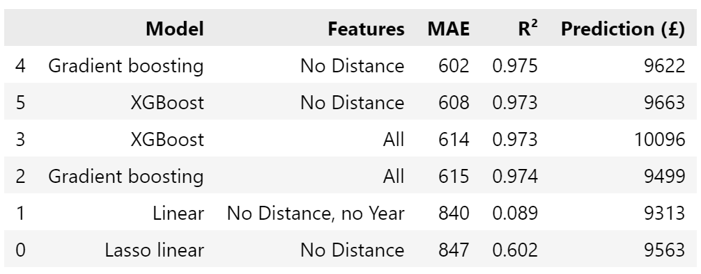
The mean of the six is £9626 - amazingly close to the top-ranked model.

Conclusion

Discussion

Clearly, the regressions using the full dataset were better, both in terms of MAE, and definitely in terms of R². This is likely due to the size of the dataset.

Scores were better without Distance, which is statistically insignificant.

A prediction of £9600 with an MAE of £600 is not great - it means a car truly priced at £9600 could be predicted as £9000 or £10,200, which is quite a large range.

Referring back to the plots from the exploratory data analysis, the line suggested ~£9450±450… So, we did lots of analysis, and didn’t really learn much more than the simple check!

Improvements

It would be great to have more features to use. Obvious ones that come to mind are paint colour, service history, number of previous owners, amount of work needed (if any), factory-fitted upgrades (e.g. rear-view camera), and aftermarket modifications. However, getting this data would not be simple, as it’s often not included on Auto Trader, so would either require a lot of extra searching using additional resources, or would result in a lot of missing data. I don’t need that much precision for this project, so I opted against it.

Another idea would be to use data from all Ford Fiestas, not just the ST-2s and ST-3s. However, there are over 10,000 currently on Auto Trader - which, using my manual scraping method, would take a long time, and would need a number of tweaks to the script to properly extract the model variant, of which there are dozens.

Actions

Before setting the price, there are some other considerations, ones related to using the result of the analysis.

First is the Auto Trader filtering mechanism. Their searching provides options for prices up to £9500, or £10,000. Asking for £10,001 means anyone filtering up to £10k wouldn’t see the car. As a prediction of ~£9600, this doesn’t affect me much, as I won’t be under £9500, and will be under £10k. Still worth checking.

Another is human psychology and pricing. What number looks good? There’s a reason almost every price tag ends in 99 - because it looks smaller. Would asking the exact predicted price - £9622 - look precise, or strange? Is £9699 better? Or, given this is a hot hatch often wanted by young men, does than number have immature connotations? Perhaps £9649 is good.