Customer Analysis Part II: Classification
This is part two of a multi-part series. Part one, segmentation and clustering, can be found here.
Code for this section can be found in the repo: https://github.com/jamesdeluk/data-science/blob/main/Projects/customer-analysis/ca2-classification.ipynb
Intro
Great, we have our customers clustered! But, hopefully, over time, we’ll gain more customers, and they’ll need to be assigned to an existing cluster. This is called classification. There are a few techniques for doing this.
First, let’s remind ourselves what our current clusters look like by grouping the data and finding the means, as we did in part one:
| Cluster | Sex | Marital status | Age | Education | Income | Occupation | Settlement size |
|---|---|---|---|---|---|---|---|
| 1 | 0.496 | 0.513 | 34.619 | 1.000 | 115413.1 | 0.825 | 0.716 |
| 2 | 0.559 | 0.536 | 31.907 | 0.898 | 81766.74 | 0.239 | 0.214 |
| 3 | 0.312 | 0.446 | 40.703 | 1.193 | 152156.7 | 1.228 | 1.216 |
| 4 | 0.291 | 0.4.000 | 44.727 | 1.345 | 223444.6 | 1.745 | 1.455 |
Now we need some new customers. I decided to make one customer for each cluster who is as close to the average as possible (within reason), to test our classification techniques. I created another who is the overall mean of the dataset (from describe()). I also made up three personas, and set the values myself (a young, unmarried, career-focussed woman; an old married educated man with an unsuccessful career; and a young unmarried urban man with an unsuccessful career). Finally, I used random to create three random customers.
df_new_customers = pd.DataFrame([
{'ID':100002001,'Sex':0,'Marital status':1,'Age':35,'Education':1,'Income':115000,'Occupation':1,'Settlement size':1}, # expect 1
{'ID':100002002,'Sex':1,'Marital status':1,'Age':32,'Education':1,'Income':82000,'Occupation':0,'Settlement size':0}, # expect 2
{'ID':100002003,'Sex':0,'Marital status':0,'Age':41,'Education':1,'Income':152000,'Occupation':1,'Settlement size':1}, # expect 3
{'ID':100002004,'Sex':0,'Marital status':0,'Age':45,'Education':1,'Income':223000,'Occupation':2,'Settlement size':1}, # expect 4
{'ID':100002005,'Sex':0,'Marital status':0,'Age':36,'Education':1,'Income':121000,'Occupation':1,'Settlement size':1}, # dataset mean
{'ID':100002006,'Sex':1,'Marital status':0,'Age':31,'Education':2,'Income':120000,'Occupation':1,'Settlement size':2}, # young unmarried career-focussed woman
{'ID':100002007,'Sex':0,'Marital status':1,'Age':50,'Education':2,'Income':90000,'Occupation':0,'Settlement size':0}, # old married man with education but little career
{'ID':100002008,'Sex':0,'Marital status':0,'Age':28,'Education':0,'Income':90000,'Occupation':0,'Settlement size':2}, # young unmarried man with unsuccessful career in a big city
{'ID':100002009,'Sex':random.randint(0,1),'Marital status':random.randint(0,1),'Age':random.randint(18,70),'Education':random.randint(0,3),'Income':random.randint(30000,300000),'Occupation':random.randint(0,2),'Settlement size':random.randint(0,2)}, # random
{'ID':100002010,'Sex':random.randint(0,1),'Marital status':random.randint(0,1),'Age':random.randint(18,70),'Education':random.randint(0,3),'Income':random.randint(30000,300000),'Occupation':random.randint(0,2),'Settlement size':random.randint(0,2)}, # random
{'ID':100002011,'Sex':random.randint(0,1),'Marital status':random.randint(0,1),'Age':random.randint(18,70),'Education':random.randint(0,3),'Income':random.randint(30000,300000),'Occupation':random.randint(0,2),'Settlement size':random.randint(0,2)}, # random
]).set_index('ID')
Which gave me:
| ID | Sex | Marital status | Age | Education | Income | Occupation | Settlement size |
|---|---|---|---|---|---|---|---|
| 100002001 | 0 | 1 | 35 | 1 | 115000 | 1 | 1 |
| 100002002 | 1 | 1 | 32 | 1 | 82000 | 0 | 0 |
| 100002003 | 0 | 0 | 41 | 1 | 152000 | 1 | 1 |
| 100002004 | 0 | 0 | 45 | 1 | 223000 | 2 | 1 |
| 100002005 | 0 | 0 | 36 | 1 | 121000 | 1 | 1 |
| 100002006 | 1 | 0 | 31 | 2 | 120000 | 1 | 2 |
| 100002007 | 0 | 1 | 50 | 2 | 90000 | 0 | 0 |
| 100002008 | 0 | 0 | 28 | 0 | 90000 | 0 | 2 |
| 100002009 | 0 | 0 | 58 | 0 | 284597 | 0 | 1 |
| 100002010 | 1 | 1 | 21 | 3 | 151823 | 2 | 2 |
| 100002011 | 1 | 1 | 64 | 2 | 107499 | 2 | 0 |
Of course, unless I save this, every time I re-run the code, the random customers will change. Currently we have a unmarried old man with a very high income yet no education or occupation (investments?), a young married woman in a big city who already has a PhD and a managerial job whose income hasn’t caught up yet (very impressive), and an old married woman who is educated and in a managerial job earning a small-city income.
OK, we have our new customers. Final pre-processing involves rescaling the existing customer data and the new customer data, and preparing to capture the results by creating a DataFrame called results.
Plots
You know I like visuals. I forgot about the Seaborn’s jointplot in part one - it’s a scatter, but with the distributions:
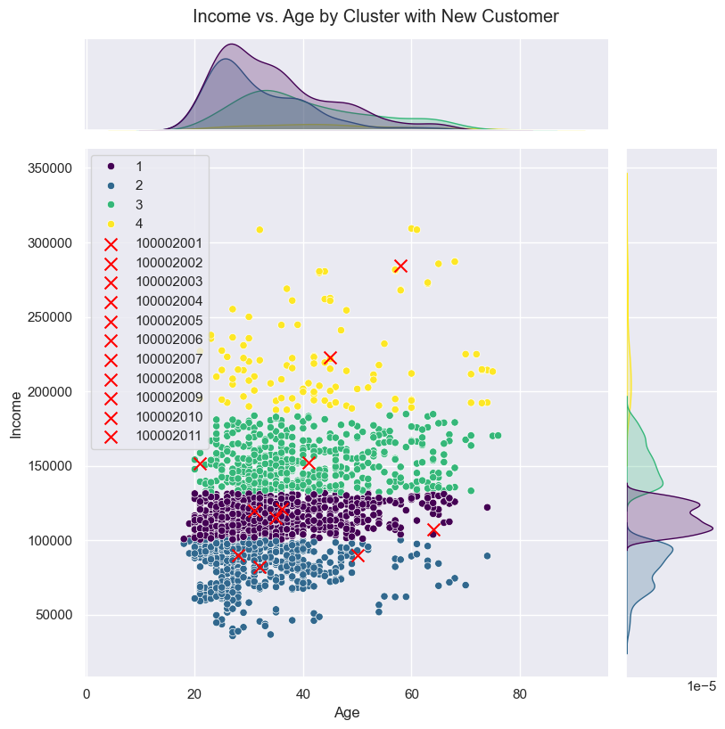
We can see income is quite nicely split in our clustering method, but age has a lot of overlaps.
Anyway, based on this plot - which only covers two of the seven features - our various users are split amongst the clusters, which means hopefully we’ll get a range of predictions.
What if do extend this to all features? Seaborn does have a pairplot function, but it doesn’t easily enable adding the new points, so I made one myself using loops. Unfortunately (but unsurprisingly):
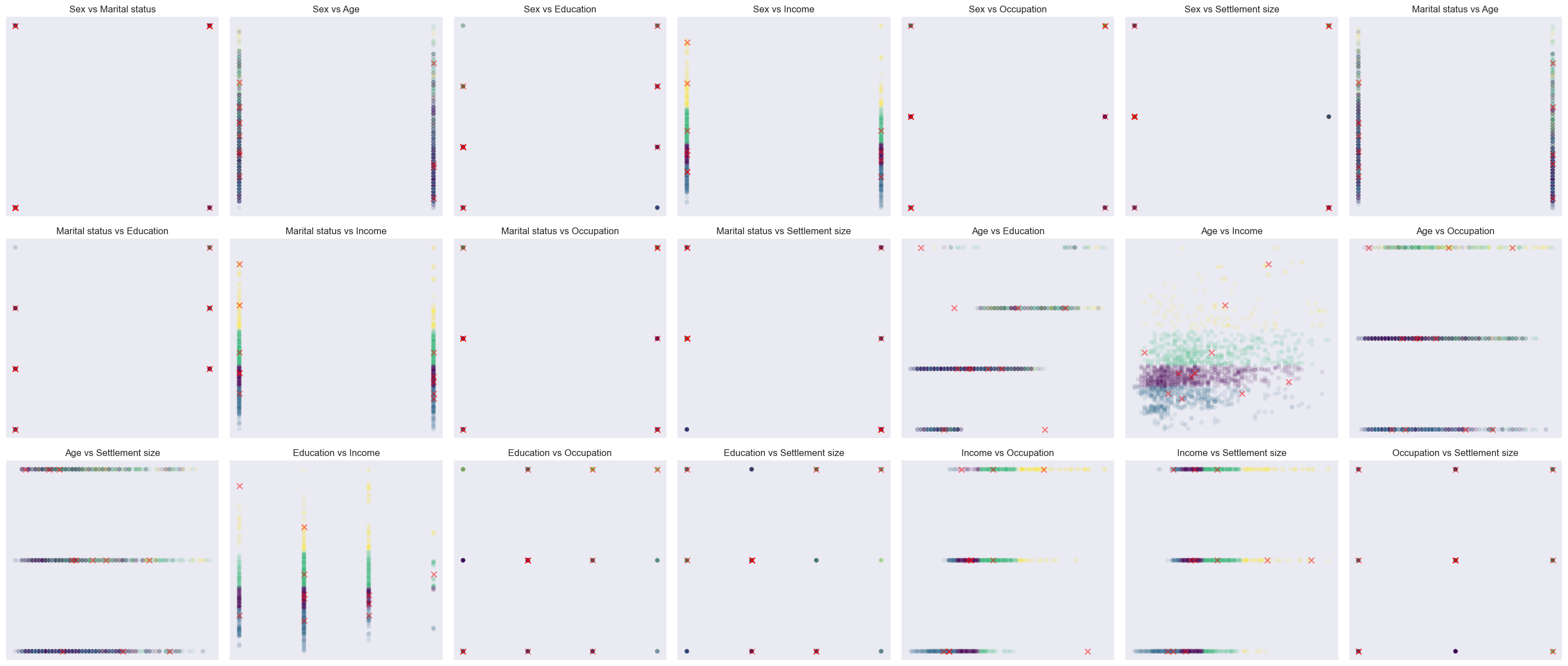
It’s a bit of a mess (open the image in a new tab to zoom in). I made the core points transparent to try and get the “main” colour to show through, but it’s hard to see, especially the categoricals. I realise all the customers are the same red X, but trust me, even if I made them different, there’s little we can gain from this.
I guess we’ll have to do it technically.
Techniques
To save repetition, I’ve only included the key code snippets below; none of the bits which print the results to screen or record them to the results DataFrame mentioned above. If you want it, it’s in the repo.
Re-cluster
The simple method is to simply repeat the original clustering process, but include the new data.
First I needed a new DataFrame with the old and new data:
df_customers_including_new = pd.concat([df_customers.drop('Cluster', axis=1), df_new_customers])
Then I copied the hierarchical clustering code from part one and re-ran it. We get:
New customer 100002001 assigned to cluster 1
New customer 100002002 assigned to cluster 2
New customer 100002003 assigned to cluster 3
New customer 100002004 assigned to cluster 4

New customer 100002005 assigned to cluster 1

New customer 100002006 assigned to cluster 1
New customer 100002007 assigned to cluster 2
New customer 100002008 assigned to cluster 2

New customer 100002009 assigned to cluster 4
New customer 100002010 assigned to cluster 3
New customer 100002011 assigned to cluster 1
That actually looks decent - the first four are as expected, and the others are spread across the four clusters. We don’t know how accurate this is yet, but it seems good!
But there are a few problems with this approach.
One is scalability. Hierarchical clustering has a Big O of O(n³), with n being the number of datapoints - that means the complexity of the operation increases rapidly with the size of the dataset, and hence it cannot handle large datasets. The maths doesn’t quite work this way, but for 10 datapoints, the complexity is 10³ = 1000, but with 100 it’s 10³ = 1,000,000 - in other words, 10x more datapoints makes it 1000x more complex. Doing this once may be okay, but re-doing it for every new customer… Not feasible.
There is another issue with re-clustering, but we’ll see that later…
Distance to cluster centroids
OK, on to classification techniques. The first one is distance to cluster centroids. It calculates the centre of each cluster, and sees to which the new datapoint is closest.
df_centroids = df_customers_features.groupby(df_customers_clusters).mean()
df_centroids_scaled = scaler.transform(df_centroids)
for i, new_customer in enumerate(df_new_customers_scaled):
    distances = np.linalg.norm(df_centroids_scaled - new_customer, axis=1)
    assigned_cluster = df_centroids.index[np.argmin(distances)]
This gives:
New customer 100002001 assigned to cluster 1
New customer 100002002 assigned to cluster 2
New customer 100002003 assigned to cluster 3
New customer 100002004 assigned to cluster 4

New customer 100002005 assigned to cluster 1

New customer 100002006 assigned to cluster 3
New customer 100002007 assigned to cluster 2
New customer 100002008 assigned to cluster 1

New customer 100002009 assigned to cluster 4
New customer 100002010 assigned to cluster 3
New customer 100002011 assigned to cluster 3
The first four match our expectations, which is a good sign. Many of the rest rest, however, are different from the re-clustering technique.
Rather than go into detail now, I’ll do so later, once we have the results from all the techniques in a single table.
Taking a step back, is this technique likely to be reliable? Possibly… But possible not. We used hierarchical clustering to create the original clusters. Hierarchical clustering is distance-based, as we saw with the dendrogram in part one, and hence isn’t designed to have “good” cluster centroids, something this method of classification relies upon. Let’s try more techniques.
K-nearest neighbours (KNN)
This is distance-based, but it still relies on centroids and spherical clusters - as the name suggests, it’s great for K-based clustering, like K-means, but may have the same issues as distance to cluster centroids when classifying into hierarchically clustered data. But it’s a popular technique, so I wanted to give it a go anyway, even if it proves to be not particularly useful for us. There are two ways I’ll approach this - stability / majority, and optimal.
Stability / majority
For the first approach, I’ll loop through a range of parameters - number of neighbours and weights - and see which the new customer is most commonly assigned to, with the percentage of how many of the loops assigned that cluster:
for i, new_customer in enumerate(df_new_customers_scaled):
    knn_assignment = []
    for n in range(1,101):
        for w in ['uniform', 'distance']:
            knn = KNeighborsClassifier(n_neighbors=n, weights=w)
            knn.fit(df_customers_features_scaled, df_customers_clusters)
            assigned_cluster_knn = knn.predict(new_customer.reshape(1, -1))
            knn_assignment.append(int(assigned_cluster_knn[0]))
    assignment_counts = Counter(knn_assignment)
    max_n = max(assignment_counts.values())
    top_clusters = [(c, n) for c, n in assignment_counts.items() if n == max_n]
How many neighbours? A good rule of thumb is the square root of the total number of datapoints. We have 2000 rows, the square root of which is 45, so I thought 1 to 100 is a good range.
We get:
New customer 100002001 assigned to cluster 1 (100.0%)
New customer 100002002 assigned to cluster 2 (100.0%)
New customer 100002003 assigned to cluster 3 (83.0%)
New customer 100002004 assigned to cluster 4 (73.0%)

New customer 100002005 assigned to cluster 1 (100.0%)

New customer 100002006 assigned to cluster 1 (100.0%)
New customer 100002007 assigned to cluster 2 (99.5%)
New customer 100002008 assigned to cluster 1 (55.0%)

New customer 100002009 assigned to cluster 3 (54.0%)
New customer 100002010 assigned to cluster 3 (100.0%)
New customer 100002011 assigned to cluster 3 (73.0%)
The first four look pretty good, but many of the others are different from the cluster centroids technique. Also, 2008 only has a ~55% confidence of being cluster 1, and 2009 has only 54%, which doesn’t inspire us with confidence.
Optimal
The other method, optimal, uses a grid search and cross validation to find the parameters (again, number of neighbours and weights) which results in the best score, based on accuracy:
parameters = {'n_neighbors': range(1, 101), 'weights': ['uniform', 'distance']}
grid_search_knn = GridSearchCV(estimator=KNeighborsClassifier(), param_grid=parameters, scoring='accuracy', cv=5)
grid_search_knn.fit(df_customers_features_scaled, df_customers_clusters)

for i, new_customer in enumerate(df_new_customers_scaled):
    assigned_cluster_knn = grid_search_knn.best_estimator_.predict(pd.DataFrame([new_customer]))
The best score was 0.8715, with (kind of strangely) only one neighbour and uniform weights. The first five are the same, but:
New customer 100002006 assigned to cluster 1
New customer 100002007 assigned to cluster 2
New customer 100002008 assigned to cluster 2

New customer 100002009 assigned to cluster 4
New customer 100002010 assigned to cluster 3
New customer 100002011 assigned to cluster 3
Similar to the majority method, but not exactly - both 2008 and 2009, the low % ones, have jumped to a different cluster.
Random forest
This might be a better idea. As previously mentioned, hierarchical clustering is distance-based, which is more similar to how decision trees work. I used decision trees in predicting the price of my car (see the post here), but decision trees can also be used for classification. I started with a basic one, with all defaults, only setting random_state to ensure repeatability:
rf = RandomForestClassifier(random_state=42)
rf.fit(df_customers_features, df_customers_clusters)
for _, new_customer in df_new_customers.iterrows():
    assigned_cluster_rf = rf.predict(pd.DataFrame([new_customer], columns=df_customers_features.columns))
Again, the first five are the same, as are my personas, but two of the three randoms have been assigned differently:
New customer 100002009 assigned to cluster 3
New customer 100002010 assigned to cluster 3
New customer 100002011 assigned to cluster 1
Similar to the car pricing project, we can use BayesSearchCV to find the optimum parameters for the classification. This is a non-exhaustive list of parameters, but should do a reasonable job:
ss_rf = {
    'n_estimators': (50 , 300),
    'max_depth': (1, 30, None),
    'min_samples_split': (2, 20),
    'min_samples_leaf': (1, 20),
    'bootstrap': [True, False],
    'max_features': ['sqrt', 'log2', None],
}
bayes_search_rf = BayesSearchCV(estimator=RandomForestClassifier(random_state=42), search_spaces=ss_rf, n_iter=100, scoring='accuracy', cv=5)
bayes_search_rf.fit(df_customers_features, df_customers_clusters)

for _, new_customer in df_new_customers.iterrows():
    assigned_cluster_rf = bayes_search_rf.best_estimator_.predict(pd.DataFrame([new_customer], columns=df_customers_features.columns))
The best parameters:
Best score: 1.0
Best parameters: OrderedDict({'bootstrap': False, 'max_depth': 30, 'max_features': None, 'min_samples_leaf': 15, 'min_samples_split': 6, 'n_estimators': 256})
Somehow a best score of 1.0 sees too high - is anything ever perfect? Something to consider.
The only difference in clustering was that one of the random customers has changed:
New customer 100002009 assigned to cluster 4
I also thought to test it with scaled data, as sometimes that can be useful when a dataset contains mixed data, as ours does:
Best score: 1.0
Best parameters: OrderedDict({'bootstrap': False, 'max_depth': None, 'max_features': None, 'min_samples_leaf': 1, 'min_samples_split': 5, 'n_estimators': 70})
Same best score, but different parameters. Same outcome as the unscaled Bayes search though.
Random forests are also able to give you feature importance statistics - that is, out of the different columns, which have the biggest impact on the classification. These statistics are typically more reliable on scaled data, as our last Bayes search was, as that can remove the influence of features with dramatically different magnitudes (as we have). What do we find?
| Feature | RF | Bayes | Scaled Bayes |
|---|---|---|---|
| Sex | 0.006 | 0.0 | 0.0 |
| Marital status | 0.004 | 0.0 | 0.0 |
| Age | 0.048 | 0.0 | 0.0 |
| Education | 0.015 | 0.0 | 0.0 |
| Income | 0.779 | 1.0 | 1.0 |
| Occupation | 0.103 | 0.0 | 0.0 |
| Settlement size | 0.046 | 0.0 | 0.0 |
It seems Income is by far the most important feature - literally, Income has an importance of 1, whereas all the others have 0, with “optimum” parameters. Which is a tad suspicious, especially combined with the parameter best score of 1.0. Maybe we’ll look into this later.
XGBoost
Another tree-based model, often seen as slightly better (if more complex) than random forests:
xgb = XGBClassifier(random_state=42)
xgb.fit(df_customers_features, df_customers_clusters-1)
for _, new_customer in df_new_customers.iterrows():
    predicted_cluster_xgb = xgb.predict(pd.DataFrame([new_customer], columns=df_customers_features.columns))
This gave the same results as the Bayes-searched random forests.
I also did a Bayes search for this, and another for scaled data:
Best score: 0.997
Best parameters: OrderedDict({'colsample_bytree': 0.5787369657850708, 'learning_rate': 0.3454416614755435, 'max_depth': 2, 'n_estimators': 241, 'reg_alpha': 0.684240056451956, 'reg_lambda': 3, 'subsample': 0.6933880726543628})
Best score: 0.997
Best parameters: OrderedDict({'colsample_bytree': 0.5292632619794049, 'learning_rate': 0.4164540777581422, 'max_depth': 2, 'n_estimators': 243, 'reg_alpha': 0.14394864350923378, 'reg_lambda': 10, 'subsample': 0.7008387947608258})
The score is slightly lower, but therefore possibly more believable. Same clustering results as before.
As for the feature importances, for the defaults, Income had an importance of 0.99, but after the Bayes searches, we have what looks to me as a better outcome:
| Feature | XGB | Bayes | Scaled Bayes |
|---|---|---|---|
| Income | 0.9902 | 0.0005 | 0.0274 |
| Settlement size | 0.0036 | 0.0021 | 0.0205 |
| Age | 0.0026 | 0.0148 | 0.0573 |
| Marital status | 0.0024 | 0.0320 | 0.0302 |
| Sex | 0.0006 | 0.4145 | 0.5179 |
| Occupation | 0.0003 | 0.4318 | 0.2755 |
| Education | 0.0002 | 0.1044 | 0.0712 |
Focussing on the scaled one, for reasons given earlier:
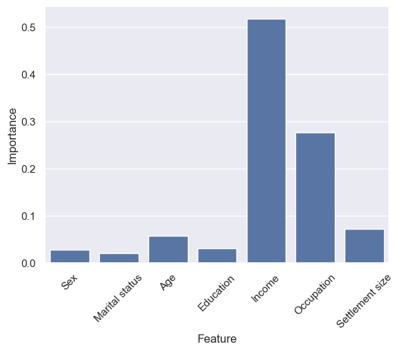
Income is still the most important, but Occupation has a reasonably large effect this time too. Marital status has the lowest impact. Given this is customers buying products from a store, this doesn’t surprise me - income is a major factor in how much a customer purchases, so it makes sense that typically high-income and low-income customers would be grouped together more than married and unmarried.
Logistic regression
Final one, a logistic regression. It uses a linear combination of the column values to classify. We might see this more in future parts of this project. Anyway:
lr = LogisticRegression(random_state=42)
lr.fit(df_customers_features_scaled, df_customers_clusters)
for i, new_customer in enumerate(df_new_customers_scaled):
    predicted_cluster_lr = lr.predict(pd.DataFrame([new_customer]))
The same results. Again. And another Bayes hyperparameter search:
Best score: 0.9935
Best parameters: OrderedDict({'C': 74.52328479283184, 'penalty': 'l2', 'solver': 'lbfgs'})
Another very high score, with the same clustering results.
While LogRegs don’t have feature importances, they have the per-cluster coefficients used in the linear combination, which works as a proxy for feature importances. Focussing on the tuned model (the default model is only slightly different):
| Cluster | Sex | Marital status | Age | Education | Income | Occupation | Settlement size | Intercept |
|---|---|---|---|---|---|---|---|---|
| 1 | -0.078 | -0.072 | -0.132 | 0.073 | -11.466 | -0.018 | 0.092 | 19.731 |
| 2 | -0.239 | 0.473 | 0.338 | -0.386 | -54.724 | -0.044 | 0.042 | -3.716 |
| 3 | 0.013 | 0.040 | 0.058 | -0.007 | 22.805 | -0.104 | 0.188 | 9.595 |
| 4 | 0.304 | -0.441 | -0.264 | 0.320 | 43.385 | 0.165 | -0.321 | -25.610 |
A positive number means a positive correlation, a negative a negative. We can see, for example, cluster 4 has a strong positive correlation with Income, whereas cluster 2 has a strong negative correlation. Similar to the decision trees, overall, Income is by far the biggest factor in which cluster a customer will be assigned to. Excluding Income, based absolute values, this time it seems Marital status has the second-highest impact (0.256), with Occupation the lowest (0.008). It’s interesting how the techniques can be quite different under the bonnet, but still produce the same outcomes! As for the Intercept, this suggests the “default” group is cluster 1, as it has the highest value, and cluster 4 is the least likely for a customer to be in, which roughly correlates to size of each group (cluster 1 is the largest, cluster 4 the smallest).
Results
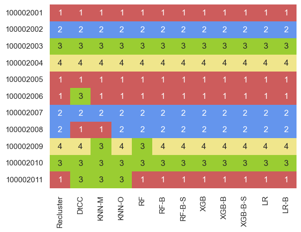
Our final results, in a nice visual heatmap (albeit not one representing scales or magnitudes like a typical heatmap), look like:
If we want some stats, such as the mean and mode, we can:
results_mean = pd.DataFrame(results.T.mean()).round(2).rename(columns={0:'Mean'})
results_mode = pd.DataFrame(results.T.agg(lambda x: x.mode()[0])).rename(columns={0:'Mode'})
pd.merge(left=results_mean, right=results_mode, left_index=True, right_index=True)
We get:
| ID | Mean | Mode |
|---|---|---|
| 100002001 | 1 | 1 |
| 100002002 | 2 | 2 |
| 100002003 | 3 | 3 |
| 100002004 | 4 | 4 |
| 100002005 | 1 | 1 |
| 100002006 | 1.15 | 1 |
| 100002007 | 2 | 2 |
| 100002008 | 1.85 | 2 |
| 100002009 | 3.85 | 4 |
| 100002010 | 3 | 3 |
| 100002011 | 1.46 | 1 |
Assessment
Our first five, our test customers and the overage dataset average, were all classified the same by all the models. This is a good sign - none of them are going crazy, and they all agree with the re-clustering technique.
For my personas, there was mostly agreement, although there were overall three differences - distance to cluster centroids method for 2006, and distance to cluster centroids and KNN majority-based for 2008.
Of the randoms, 2010 had universal agreement, whereas 2009 had two of disagreers (KNN-M and random forest) and 2011 had three (distance to cluster centroids, KNN-M and KNN-O). This is not surprising, as some of the randomly-generated customers have a higher chance of being dissimilar to a real customer, a higher chance of being outliers.
All this put a different way, relative to the re-clustering or mode result, RF and KNN-O had one difference each, and distance to cluster centroids and KNN-M had three differences.
Based on this, we can’t easily tell which technique is best. If we use the re-clustering technique as the most accurate, given it’s using the same logic as the original clustering, the techniques that gave the same results were tuned random forest, XGB (tuned and defaults), and logistic regressions (tuned and defaults). This would make sense, as, as mentioned earlier, tree-based techniques are more similar to how hierarchical clustering functions. The unusual best score and feature importances for random forest make me a tad wary, as with the untuned making “errors”, which would make me more inclined to use XGB and LogReg for this client.
There is one thing to be aware of. Tree-based techniques can be more computationally expensive, especially doing the hyperparameter tuning - for example, the distance to cluster centroids approach took 0.0 seconds, but the random forest Bayes search took almost 13 minutes! Once the parameters are found and the model is tuned, the actual classification took under a second. Even so, similar to re-clustering, as the dataset grows, parameters will need to be retuned.
A different dataset
I’ve mentioned a few times that we expected a tree-based technique to be best for hierarchically clustered data, as ours was. But what if it wasn’t?
The joys of code is you only need to change a few lines to do everything for a different dataset! In part one we clustered with K-prototypes, and it was scored as the second best after hierarchical clustering. What about repeating all the above, but for a different clustering technique?
In part one we only had three clusters for K-prototypes, but let’s make one with four, so it’s easier to compare. I’ll use the same random customers though. Also, the four average-per-cluster customers will be different, as this dataset has different means.
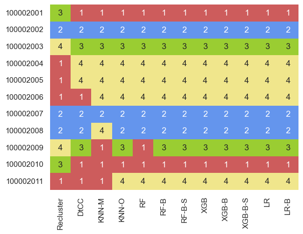
The results:
And the stats:
| ID | Mean | Mode |
|---|---|---|
| 100002001 | 1.17 | 1 |
| 100002002 | 2.00 | 2 |
| 100002003 | 3.08 | 3 |
| 100002004 | 3.75 | 4 |
| 100002005 | 3.75 | 4 |
| 100002006 | 3.50 | 4 |
| 100002007 | 2.00 | 2 |
| 100002008 | 2.17 | 2 |
| 100002009 | 2.75 | 3 |
| 100002010 | 1.17 | 1 |
| 100002011 | 3.25 | 4 |
I’ll get to the re-cluster column in a bit, but first, let’s look at the results. Given K-prototypes generates cluster centroids, we’d imagine the distance to cluster centroids and KNN might perform better than the tree-based or logistic regression techniques, or at least on par.
As before, all the techniques agree on our average-based customers, which is good. Also as before, all the tree-based techniques (excluding the basic random forest) and logistic regression agree, although in this case, the optimum-based KNN model also agrees with these. On the other hand, the random forest has one difference (2009), distance to cluster centroids has two differences (2010, 2011), and KNN majority-based has three differences (2008, 2009, 2011).
The best score for the random forest was again 1, and Income again had a feature importance of 1. XGBoost, score of 0.998, with the top three features again being Income (0.73), Occupation (0.16), and Settlement size (0.06). LogReg similarly had Income as by far the most important coefficient, this time followed by Education and Occupation.
Which is best? I’m still partial to tree-based techniques, and in this case, given they agree with a KNN method, I’d opt for one of those. I’d likely pick KNN-O, XGBoost, and LogReg, and compare how they do on future new customers, prioritising the fastest and least computationally-expensive technique.
Going back to that re-clustering weirdness. There’s a major issue with re-clustering which we didn’t experience with the hierarchical dataset above - although I had experienced it in early stages of this project with different new customers. Sometimes, when re-clustering, it doesn’t just add new datapoints to an existing cluster; new datapoints (even if just a single one!) could completely change the clustering results. This is what happened here. The original dataset looked like (sorted by #):
| Cluster | Sex | Marital status | Age | Education | Income | Occupation | Settlement size | # | % |
|---|---|---|---|---|---|---|---|---|---|
| 4 | 0.51 | 0.53 | 34.43 | 1.00 | 114888.4 | 0.83 | 0.71 | 954 | 0.48 |
| 2 | 0.54 | 0.51 | 32.22 | 0.90 | 79196.03 | 0.16 | 0.16 | 486 | 0.24 |
| 1 | 0.30 | 0.44 | 40.94 | 1.19 | 154237.2 | 1.25 | 1.24 | 455 | 0.23 |
| 3 | 0.29 | 0.40 | 44.59 | 1.34 | 225124.9 | 1.77 | 1.47 | 105 | 0.05 |
But after re-clustering with the eleven new customers, the dataset became:
| Cluster | Sex | Marital status | Age | Education | Income | Occupation | Settlement size | # | % |
|---|---|---|---|---|---|---|---|---|---|
| 1 | 0.49 | 0.52 | 35.10 | 1.03 | 116796.5 | 0.85 | 0.75 | 975 | 0.48 |
| 2 | 0.55 | 0.52 | 32.19 | 0.90 | 80614.54 | 0.20 | 0.20 | 528 | 0.26 |
| 3 | 0.30 | 0.44 | 40.80 | 1.19 | 158721.7 | 1.30 | 1.24 | 424 | 0.21 |
| 4 | 0.24 | 0.37 | 44.52 | 1.30 | 234614.9 | 1.79 | 1.52 | 84 | 0.04 |
The most dramatic difference can be seen by looking at the Cluster column - they’ve changed number! 4 became 1, 1 became 3, and 3 became 4. The actual stats changed too, albeit slightly. However, this could be nightmare, as each cluster would have to be renamed and reprofiled - as it’s not just the names changing, but looking at the counts in # , some customers must also have changed cluster. So re-clustering for every new customer is definitely not a good idea.
Conclusion
Classifying a new customer is definitely better, faster, and safer than re-clustering the whole dataset.
Which technique is best really depends on how the dataset was created and knowing which technique is best for each situation. That said, I was surprised how well a bunch of the techniques worked.
I’m definitely a fan of tree-based techniques, and seem to perform well on a range of data types. They’d be my default, but it’s always worth checking other techniques depending on the data, and potentially using a combination approach. For example, logistic regression is the most explainable, if that’s important, and in this case it performed excellently.
