Analysing DVLA Data for Vintage Comebacks
GitHub repo: https://github.com/jamesdeluk/data-projects/tree/main/dvla-vehicle-statistics
Intro
The DVLA website provides vehicle licensing data, updated every few months. As a car and data enthusiast, I wanted to have a poke around. I started with two primary questions:
- What are the most popular vehicles in the UK?
- Which old vehicles are having a comeback? → This might suggest they will appreciate in value!
Selecting the dataset
There are a few different datasets, available here: https://www.gov.uk/government/statistical-data-sets/vehicle-licensing-statistics-data-files
The one(s) I decided to use were:
df_VEH0124_AM: Vehicles at the end of the year by licence status, body type, make (A to M), generic model, model, year of first use and year of manufacture: United Kingdom
Scope: All licensed vehicles in the United Kingdom with Make starting with A to M; annually from 2014
Schema: BodyType, Make, GenModel, Model, YearFirstUsed, YearManufacture, LicenceStatus, [number of vehicles; 1 column per year]
and
df_VEH0124_NZ: Vehicles at the end of the year by licence status, body type, make (N to Z), generic model, model, year of first use and year of manufacture: United Kingdom.
Scope: All licensed vehicles in the United Kingdom with Make starting with N to Z; annually from 2014
Schema: BodyType, Make, GenModel, Model, YearFirstUsed, YearManufacture, LicenceStatus, [number of vehicles; 1 column per year]
This includes everything I need, although it only goes back a decade. Another dataset does go back to 1994:
df_VEH0120_GB: Vehicles at the end of the quarter by licence status, body type, make, generic model and model: Great Britain
Scope: All registered vehicles in Great Britain; from 1994 Quarter 4 (end December)
Schema: BodyType, Make, GenModel, Model, Fuel, LicenceStatus, [number of vehicles; 1 column per quarter]
This has two main drawbacks, relative to the 124 dataset:
- Rather than annual data, this has quarterly data. In theory, this sounds better, as it’s more precise; however, given the cyclicity of car buying habits across the year, it means the numbers are more like sine waves rather than smooth lines, making any forecasting or trend-detection more difficult. For my questions, there’s no benefit for having the more granular data.
- This doesn’t include year of manufacture. This means all BMW M3s are grouped together - so an E30 M3 registered in 2023 will be grouped with a brand-new G80. One is a collectable; one is not.
Pre-processing the data
The first step is to simply join the two CSVs:
data_am = pd.read_csv("df_VEH0124_AM.csv")
data_nz = pd.read_csv("df_VEH0124_NZ.csv")
data = pd.concat([data_am, data_nz], axis=0)
This is the first row:
| BodyType | Make | GenModel | Modela | YearFirstUsed | YearManufacture | LicenceStatus | 2023 | 2022 | 2021 | 2020 | 2019 | 2018 | 2017 | 2016 | 2015 | 2014 |
|---|---|---|---|---|---|---|---|---|---|---|---|---|---|---|---|---|
| Cars | ABARTH | ABARTH 124 | 124 GT MULTIAIR | 2019 | 2019 | Licensed | 5 | 5 | 5 | 6 | 6 | 0 | 0 | 0 | 0 | 0 |
What does this tell us? In 2023, five Abarth 124 GT MultiAirs built in 2019 were licensed. Same in 2022 and 2021 (presumably the same vehicles), and 6 in 2019 and 2020. Not the most popular car!
I needed to do some minor data modifications to enable future analysis:
data.loc[:,'YearFirstUsed'] = data['YearFirstUsed'].replace('[x]',0)
data['YearFirstUsed'] = data['YearFirstUsed'].astype(int)
data.loc[:,'YearManufacture'] = data['YearManufacture'].replace('[x]',0)
data['YearManufacture'] = data['YearManufacture'].astype(int)
years = ['2023','2022','2021','2020','2019','2018','2017','2016','2015','2014']
data[years] = data[years].replace('[z]',0).astype(int)
Both FirstYearUsed and YearManufactured have some values of [x] where the data was unavailable; given I’ll be doing some date-based filtering later, I need these columns to be numerical, and hence replaced the [x] with 0. Similarly, some of the year columns had values of [z], which means the data was not applicable; again, I replaced with 0.
Melting and pivoting
Now to transform the data. First, melt it, so all the years become a single column:
data_melt = data.melt(
    id_vars=['BodyType','Make','GenModel','Model','YearFirstUsed','YearManufacture','LicenceStatus'],
    var_name='Year',
    value_name='Count'
)
data_melt['Year'] = data_melt['Year'].astype(int)
This makes the Year column an object; I need it as an integer, hence the astype.
Now the data looks like:
| BodyType | Make | GenModel | Model | YearFirstUsed | YearManufacture | LicenceStatus | Year | Count |
|---|---|---|---|---|---|---|---|---|
| Cars | ABARTH | ABARTH 124 | 124 GT MULTIAIR | 2019 | 2019 | Licensed | 2023 | 5 |
Next, pivot based on the LicenseStatus, so Licensed and SORN become separate columns:
data_pivot = data_melt.pivot_table(
    index=['BodyType','Make','GenModel','Model','YearFirstUsed','YearManufacture','Year'],
    columns='LicenceStatus',
    values='Count',
    aggfunc='sum'
).reset_index()
data_pivot['Licensed'] = data_pivot['Licensed'].fillna(0)
data_pivot['SORN'] = data_pivot['SORN'].fillna(0)
Without reset_index(), the index= columns become indexes, making life more complicated. A new NaNs appeared, for when a vehicle had data for Licensed or SORN but not both - it makes sense to, at least for this anlysis, assume there were none. Now I have:
| BodyType | Make | GenModel | Model | YearFirstUsed | YearManufacture | Year | Licensed | SORN |
|---|---|---|---|---|---|---|---|---|
| Buses and coaches | AIXAM | AIXAM MODEL MISSING | MISSING | 2007 | 2007 | 2014 | 6 | 0 |
Nope, I have no idea what an Aixam is either. Apparently it’s a French microcar manufacturer. A microcar bus/coach? Maybe one of these (pic from Wikipedia):

Kinda cute. In 2014, there were six licensed, and zero SORN, of the model manufactured in 2007.
It’s also worth noting that some of the Model data is MISSING. In fact, there are 842,360 (out of 5,442,280) MISSINGs, so about 15%. 816 out of 877 Makes have at least one MISSING. So this data is not complete - although there’s not much I can do about this right now. I was curious to see the most-registered MISSING:
data_pivot[data_pivot['Model'] == 'MISSING'].sort_values('Licensed', ascending=False)
| BodyType | Make | GenModel | Model | YearFirstUsed | YearManufacture | Year | Licensed | SORN |
|---|---|---|---|---|---|---|---|---|
| Other vehicles | OTHER BRITISH | OTHER BRITISH MODEL MISSING | MISSING | 0 | 0 | 2022 | 53515 | 3540 |
Very curious.
Initial stats
What are the most-Licensed and most-SORN vehicles? The code is quite simple (just a sort_values()), so I won’t include it here, but it’s in the repo.
| BodyType | Make | GenModel | Model | YearFirstUsed | YearManufacture | Year | Licensed | SORN |
|---|---|---|---|---|---|---|---|---|
| Cars | FORD | FORD FIESTA | FIESTA ZETEC | 2014 | 2014 | 2014 | 62883 | 131 |
Not a big surprise; you see them everywhere. What about for 2023 (the latest year with data)?
| BodyType | Make | GenModel | Model | YearFirstUsed | YearManufacture | Year | Licensed | SORN |
|---|---|---|---|---|---|---|---|---|
| Cars | FORD | FORD FIESTA | FIESTA ZETEC | 2014 | 2014 | 2023 | 59497 | 466 |
The exact same car - which kinda makes sense. Over the 9 years, about 2700 have disappeared (presumably scrapped), and 300 have been SORN.
The most SORN one overall was a MISSING (Honda motorcycle, if you’re curious). Ignoring the MISSINGs:
| BodyType | Make | GenModel | Model | YearFirstUsed | YearManufacture | Year | Licensed | SORN |
|---|---|---|---|---|---|---|---|---|
| Light goods vehicles | FORD | FORD TRANSIT | TRANSIT 350 LWB | 2005 | 2005 | 2023 | 3595 | 3490 |
Good old Transit, the white van man’s favourite. Fun fact, I once spent a few months living in a Transit (yes, out of choice).
Searching the data
Searching is easily done through str.contains. Decide the column to look in, and the phrase to look for. This will show all the unique Models including that phrase, with the count:
search_col = 'Model'
search_phrase = r'FIESTA'

model_search_data = data[data[search_col].str.contains(search_phrase, case=False, na=False)]
results = model_search_data[search_col].unique()

print(model_search_data[search_col].nunique())
for i, c in enumerate(results):
    print(f"{i}: {c}")
Okay, there are 373 Fiestas. Wow. Changing the search to FIESTA ST returns “only” 58, including my old car:
7: FIESTA ST-3 TURBO
I can use this ID to get the data:
choice = 7
model_data = data[data[search_col] == results[choice]]
model_data_pivot = data_pivot[data_pivot[search_col] == results[choice]]
If I take the head() of this data:
| BodyType | Make | GenModel | Model | YearFirstUsed | YearManufacture | Year | Licensed | SORN |
|---|---|---|---|---|---|---|---|---|
| Cars | FORD | FORD FIESTA | FIESTA ST-3 TURBO | 0 | 2016 | 2014 | 0 | 0 |
| Cars | FORD | FORD FIESTA | FIESTA ST-3 TURBO | 0 | 2016 | 2015 | 0 | 0 |
| Cars | FORD | FORD FIESTA | FIESTA ST-3 TURBO | 0 | 2016 | 2016 | 0 | 0 |
| Cars | FORD | FORD FIESTA | FIESTA ST-3 TURBO | 0 | 2016 | 2017 | 0 | 0 |
| Cars | FORD | FORD FIESTA | FIESTA ST-3 TURBO | 0 | 2016 | 2018 | 0 | 0 |
I might use this data later.
Some manufactures have the same model name (especially if it’s just a number); as such, it can be better to use GenModel instead of Model for the search_col. Of course, in some cases, to get the exact data you need, you may need to search by make and model.
Licensed to SORN ratio
Moving on, I wanted to see the ratio between Licensed and SORN. A high ratio means far more vehicles are on the road than off, implying it’s popular; a low ratio, with more SORN than licensed vehicles, implies a high number of (likely older) vehicles that haven’t been destroyed, but aren’t on the road.
data_pivot["LS_Ratio"] = data_pivot["Licensed"] / data_pivot["SORN"]
data_pivot["LS_Ratio"] = data_pivot["LS_Ratio"].replace([np.inf, -np.inf], np.nan)
The second line is needed to overcome if there are no SORN counts, as a number divided by 0 is infinite. Sorting to find the max and min of this ratio gives us:
| BodyType | Make | GenModel | Model | YearFirstUsed | YearManufacture | Year | Licensed | SORN | LS_Ratio |
|---|---|---|---|---|---|---|---|---|---|
| Cars | FORD | FORD FOCUS | FOCUS ZETEC EDITION | 2017 | 2017 | 2017 | 7985 | 1 | 7985 |
| BodyType | Make | GenModel | Model | YearFirstUsed | YearManufacture | Year | Licensed | SORN | LS_Ratio |
|---|---|---|---|---|---|---|---|---|---|
| Motorcycles | DUCATI | DUCATI 900 SS | 900 SS | 0 | 1989 | 2015 | 0 | 1 | 0 |
OK, this should have been expected. Any vehicle with a single SORN will have a high ratio, and any with none licensed with have a ratio of 0 (from the infinite result of the calculation). Picking an arbitrary value of over 1000 Licensed for the low ratios:
| BodyType | Make | GenModel | Model | YearFirstUsed | YearManufacture | Year | Licensed | SORN | LS_Ratio |
|---|---|---|---|---|---|---|---|---|---|
| Motorcycles | HONDA | HONDA MODEL MISSING | MISSING | 1981 | 1981 | 2019 | 1006 | 4883 | 0.206021 |
Let’s remove the MISSINGs:
| BodyType | Make | GenModel | Model | YearFirstUsed | YearManufacture | Year | Licensed | SORN | LS_Ratio |
|---|---|---|---|---|---|---|---|---|---|
| Cars | LAND ROVER | LAND ROVER DISCOVERY | DISCOVERY TDI | 1995 | 1995 | 2018 | 1223 | 3125 | 0.39136 |
Probably a bunch of farmers with some rusty Landies.
And over 1000 SORNs for the high ratio:
| BodyType | Make | GenModel | Model | YearFirstUsed | YearManufacture | Year | Licensed | SORN | LS_Ratio |
|---|---|---|---|---|---|---|---|---|---|
| Cars | FORD | FORD FIESTA | FIESTA ZETEC CLIMATE | 2007 | 2007 | 2019 | 25694 | 1031 | 24.92144 |
Still Ford Zetecs, but the baby brother.
I wanted to calculate the LS ratio over a multi-year period. The best way to do this was the group the data (to ensure it was only the exact same vehicle, as ungrouped the 2023 data for one vehicle would be next to the 2014 data for a different vehicle), shift the column (so the LS_ratio_-1 column for year 2023 was the LS_ratio for 2022), then take the 3- and 5-year mean.
data_pivot_grouped = data_pivot.groupby(['Make','GenModel','Model','YearManufacture'])

for n in [1,2,3,4]:
    data_pivot[f'LS_Ratio_-{n}'] = data_pivot_grouped['LS_Ratio'].shift(n)
    data_pivot[f'LS_Ratio_-{n}'] = data_pivot[f'LS_Ratio_-{n}'].fillna(0)

data_pivot['LS_Ratio_Mean_5yr'] = data_pivot[['LS_Ratio', 'LS_Ratio_-1', 'LS_Ratio_-2', 'LS_Ratio_-3', 'LS_Ratio_-4']].mean(axis=1)
data_pivot['LS_Ratio_Mean_3yr'] = data_pivot[['LS_Ratio', 'LS_Ratio_-1', 'LS_Ratio_-2']].mean(axis=1)
The first result is the Aixam again (alphabetical), but that’s mostly zeros, so let’s look at a Fiesta Zetec:
| BodyType | Make | GenModel | Model | YearFirstUsed | YearManufacture | Year | Licensed | SORN | LS_Ratio | LS_Ratio_-1 | LS_Ratio_-2 | LS_Ratio_-3 | LS_Ratio_-4 | LS_Ratio_Mean_5yr | LS_Ratio_Mean_3yr |
|---|---|---|---|---|---|---|---|---|---|---|---|---|---|---|---|
| Cars | FORD | FORD FIESTA | FIESTA ZETEC | 2014 | 2014 | 2023 | 59497 | 466 | 127.676 | 156.426 | 178.7353 | 197.1974 | 247.8992 | 181.5868 | 154.2791 |
Looks like the LS ratio is decreasing over time, and is currently below the 3- and 5-year mean, suggesting more are being SORN (or, if SORN is constant, fewer are being Licensed).
Plots
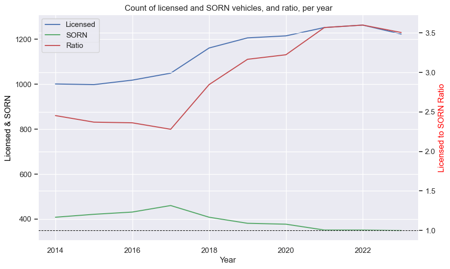
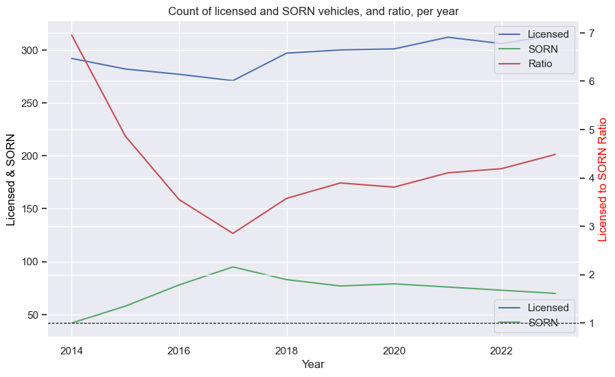
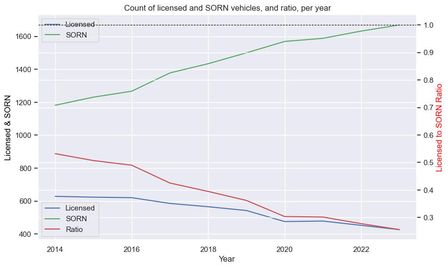
If you’ve seen any of my other posts, you know I like plots, so I built a function that plots the key values over time. The input df is best as a single car, such as from the search above. The function creates two plots. The first one is a line chart, with the Licensed and SORN counts over time on one axis, and the LS ratio on a second:
def plots(df):
    car_data_grouped_by_year = df[['Year', 'Licensed', 'SORN']]
    car_data_grouped_by_year = car_data_grouped_by_year.groupby('Year').sum()

    fig, ax1 = plt.subplots(figsize=(10,6))
    ax2 = ax1.twinx()
    plt.title("Count of licensed and SORN vehicles, and ratio, per year")

    sns.lineplot(data=car_data_grouped_by_year, x="Year", y="Licensed", ax=ax1, label="Licensed", color="b", errorbar=None, estimator=None)
    sns.lineplot(data=car_data_grouped_by_year, x="Year", y="SORN", ax=ax1, label="SORN", color="g", errorbar=None, estimator=None)
    ax1.set_ylabel("Licensed & SORN", color="black")
    ax1.set_xlabel("Year")

    car_data_grouped_by_year['LS_Ratio_Group'] = car_data_grouped_by_year['Licensed'] / car_data_grouped_by_year['SORN']

    sns.lineplot(data=car_data_grouped_by_year, x="Year", y="LS_Ratio_Group", ax=ax2, label="Ratio", color="r", errorbar=None)
    ax2.axhline(1, color='black', linewidth=0.8, linestyle='--')
    ax2.set_ylabel("Licensed to SORN Ratio", color="red")

    lines1, labels1 = ax1.get_legend_handles_labels()
    lines2, labels2 = ax2.get_legend_handles_labels()
    lines = lines1 + lines2
    labels = labels1 + labels2
    plt.legend(lines, labels, loc='best')

    plt.show()
The data needs to be grouped to get the sum by year (regardless of year of manufacture, for example). As taking the sum of the LS ratio doesn’t make sense - not any other form of aggregation, really - I recalculated it with the summed values. The legends for both axes are merged into one.
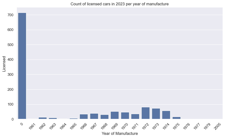
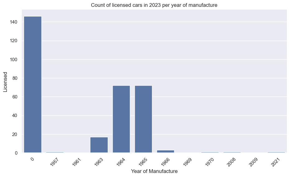
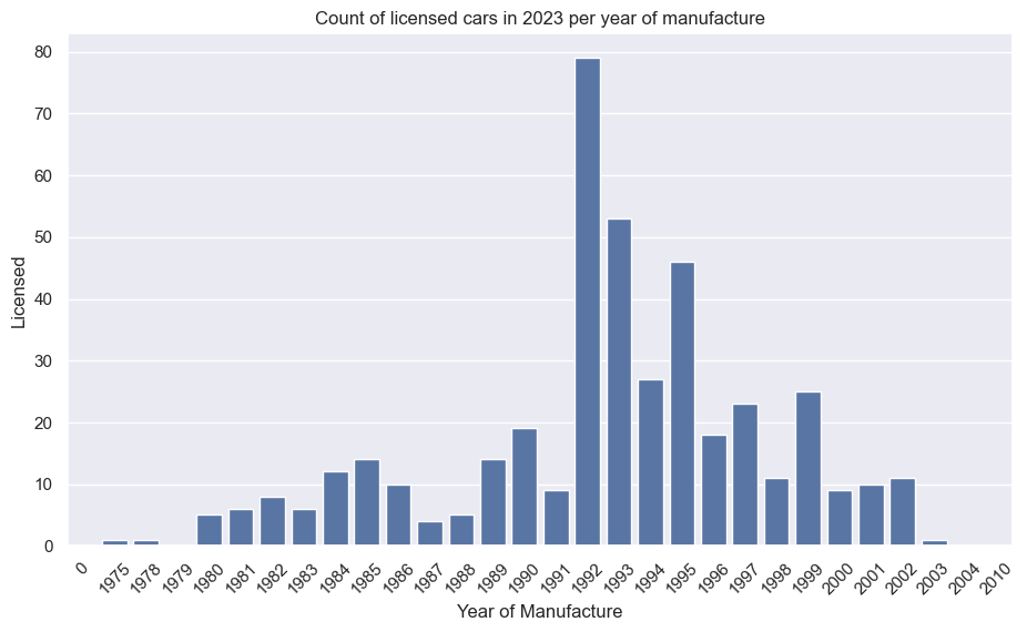
The second plot, in the same function, is a bar plot giving the number of licensed vehicles by manufacture year (again, requiring a groupby and sum):
    car_data_grouped_by_manu_year = df[df['Year'] == 2023][['YearManufacture','Licensed']].groupby('YearManufacture').sum()

    plt.figure(figsize=(11,6))
    plt.title("Count of licensed cars per year of manufacture")
    sns.barplot(car_data_grouped_by_manu_year, x=car_data_grouped_by_manu_year.index, y='Licensed')
    plt.xlabel("Year of Manufacture")
    plt.xticks(rotation=45)
    plt.show()
Using the ST-3 search example above:
plots(model_data_pivot)
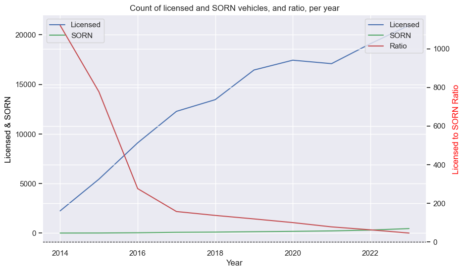
The first chart shows a steady increase licensed STs, and a slow increase in SORNs. The ratio drops dramatically at first, as expected, as a small increase in SORN results in a large percentage change (the curse of percentages).
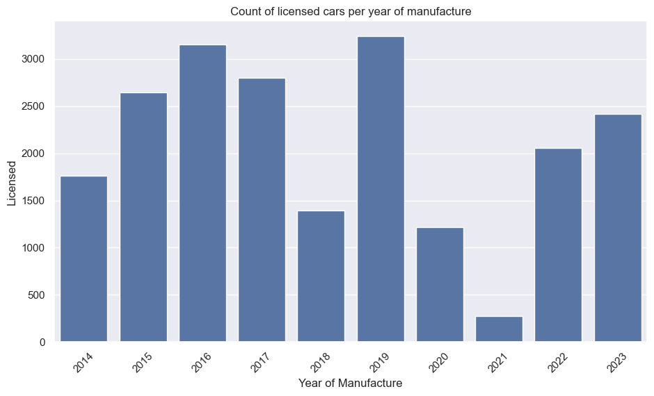
The second chart shows how 2019 was the most popular year of manufacture, with huge drops in 2020 and 2021 (thanks COVID). Side note, a new generation was released in 2017; I wonder if that could be a cause of the drop in 2018 (for example, waiting to see if the new car is good). There’s no way of separating generation in this dataset.
By adding display() into the plots() function, we can see the data used to build the plots:
| Year | Licensed | SORN | LS_Ratio_Group |
|---|---|---|---|
| 2014 | 2242 | 2 | 1121 |
| 2015 | 5440 | 7 | 777.1429 |
| 2016 | 9106 | 33 | 275.9394 |
| 2017 | 12281 | 78 | 157.4487 |
| 2018 | 13461 | 98 | 137.3571 |
| 2019 | 16454 | 138 | 119.2319 |
| 2020 | 17443 | 174 | 100.2471 |
| 2021 | 17093 | 219 | 78.05023 |
| 2022 | 19102 | 304 | 62.83553 |
| 2023 | 20959 | 455 | 46.06374 |
| YearManufacture | Licensed |
|---|---|
| 2014 | 1759 |
| 2015 | 2647 |
| 2016 | 3154 |
| 2017 | 2803 |
| 2018 | 1392 |
| 2019 | 3239 |
| 2020 | 1215 |
| 2021 | 276 |
| 2022 | 2055 |
| 2023 | 2419 |
Older vehicles
Time for a specific question. What 20th century vehicles are still on the road?
display(
    data_pivot[(data_pivot['BodyType'] != 'Motorcycles') & (data_pivot['BodyType'] != 'Light goods vehicles') & (data_pivot['BodyType'] != 'Other vehicles') & (data_pivot['YearManufacture'] < 2000) & (data_pivot['Model'] != 'MISSING') & (data_pivot['Licensed'] > 100) & (data_pivot['Year'] == 2023)]
    .drop(['Year','LS_Ratio_-1','LS_Ratio_-2','LS_Ratio_-3','LS_Ratio_-4'], axis=1)
    .sort_values('LS_Ratio_Mean_5yr', ascending=False)
    .head(5)
)
This will give cars manufactured before 2000, excluding the MISSINGs, with more than 100 licensed in 2023. Drop the unnecessary columns, and sort by the 5-year mean LS ratio:
| Make | GenModel | Model | YearFirstUsed | YearManufacture | Licensed | SORN | LS_Ratio | LS_Ratio_Mean_5yr | LS_Ratio_Mean_3yr |
|---|---|---|---|---|---|---|---|---|---|
| MG | MG MGB | B | 1981 | 1980 | 159 | 5 | 31.8 | 48.96 | 80.6 |
| MG | MG MGB | B GT | 1981 | 1980 | 164 | 5 | 32.8 | 33.52667 | 55.54444 |
| MG | MG MGB | B | 1974 | 1973 | 101 | 8 | 12.625 | 15.925 | 15.65278 |
| MG | MG MGB | B | 1966 | 1966 | 113 | 13 | 8.692308 | 9.127772 | 9.193473 |
| MG | MG MGA | A | 1959 | 0 | 171 | 22 | 7.772727 | 8.135448 | 7.689065 |
All MGs! Even now, 45 years later, there are 30 times as many MGBs on the road than are SORN. However, the 2023 LS ratio is lower than the 3- and 5-year means, suggesting more are going off the road (that said, given the SORN figure is 5, a jump from 4 to 5 would dramatically change the ratio, so the change in ratio may not be as significant as it looks).
Let’s group by the model, regardless of the year of manufacture (as long as it’s pre-2000). When grouping, you have to define how to aggregate the other columns; I’ll take the sum of Licensed and SORN (giving all the vehicles), and the mean of the ratios (as summing ratios is nonsensical):
display(
    data_pivot[(data_pivot['BodyType'] != 'Motorcycles') & (data_pivot['BodyType'] != 'Light goods vehicles') & (data_pivot['BodyType'] != 'Other vehicles') & (data_pivot['YearManufacture'] < 2000) & (data_pivot['Model'] != 'MISSING') & (data_pivot['Licensed'] > 100) & (data_pivot['Year'] == 2023)]
    .drop(['GenModel','YearFirstUsed','YearManufacture','Year','LS_Ratio_-1','LS_Ratio_-2','LS_Ratio_-3','LS_Ratio_-4'], axis=1)
    .groupby('Model', as_index=False)
    .agg({'BodyType':'first', 'Make':'first', 'Licensed':'sum', 'SORN':'sum', 'LS_Ratio':'mean', 'LS_Ratio_Mean_5yr':'mean', 'LS_Ratio_Mean_3yr':'mean'})
    .sort_values('LS_Ratio_Mean_5yr', ascending=False)
    .head(5)
)
Note how taking the mean LS ratio means it’s not the same as the sum of Licensed divided by sum of SORN - it’s typically close, but sometimes but always.
| Model | Make | Licensed | SORN | LS_Ratio | LS_Ratio_Mean_5yr | LS_Ratio_Mean_3yr |
|---|---|---|---|---|---|---|
| MINI MINOR | MORRIS | 108 | 15 | 7.2 | 6.695833 | 6.986111 |
| TR2 | TRIUMPH | 136 | 22 | 6.181818 | 6.093074 | 6.139971 |
| A | MG | 1042 | 192 | 5.757499 | 5.948549 | 5.850808 |
| MUSTANG GT | FORD | 210 | 35 | 6.238095 | 5.926916 | 6.240947 |
| B | MG | 12297 | 4302 | 4.823928 | 5.338588 | 6.451258 |
The MGs are still there, but now a Triumph joins the pack. Also, a Mustang and a Mini. For those who’ve never seen the classic Mustang-vs-Mini races, watch this:
Next, the same search, but grouping by the GenModel, giving a slightly broader view - in this query, for example, all the MGBs in the table two above would be grouped:
display(
    data_pivot[(data_pivot['BodyType'] != 'Motorcycles') & (data_pivot['BodyType'] != 'Light goods vehicles') & (data_pivot['BodyType'] != 'Other vehicles') & (data_pivot['YearManufacture'] < 2000) & (data_pivot['Model'] != 'MISSING') & (data_pivot['Licensed'] > 100) & (data_pivot['Year'] == 2023)]
    .drop(['BodyType','Model','YearFirstUsed','YearManufacture','Year','LS_Ratio_-1','LS_Ratio_-2','LS_Ratio_-3','LS_Ratio_-4'], axis=1)
    .groupby('GenModel', as_index=False)
    .agg({'Make':'first', 'Licensed':'sum', 'SORN':'sum', 'LS_Ratio_Mean_5yr':'mean', 'LS_Ratio_Mean_3yr':'mean'})
    .sort_values('LS_Ratio_Mean_5yr', ascending=False)
    .head(5)
)
| GenModel | Make | Licensed | SORN | LS_Ratio_Mean_5yr | LS_Ratio_Mean_3yr |
|---|---|---|---|---|---|
| TRIUMPH TR2 | TRIUMPH | 136 | 22 | 6.093074 | 6.139971 |
| MG MGA | MG | 1042 | 192 | 5.948549 | 5.850808 |
| FORD MUSTANG | FORD | 325 | 64 | 5.644761 | 5.678685 |
| TRIUMPH TR5 | TRIUMPH | 298 | 55 | 5.267664 | 5.602357 |
| TRIUMPH TR3 | TRIUMPH | 122 | 28 | 5.016905 | 4.644841 |
More Triumphs join the mix!
What have we learnt so far? In the UK, there are a surprising number of classic Triumphs and MGs from the 60s, 70s, and 80s still on the road - at least, relative to the ones which are parked up and not roadgoing. This doesn’t particularly surprise me - I regularly see old MGs and Triumphs. However, I didn’t expect them to be the most popular of the vintage classics.
Phoenixes
Now to focus on the second question - which old cars are having a comeback? I decided to call these phoenixes - those which died, but have come back.
Again, I was only interested in cars from the 20th century:
phoenix_data = data_pivot[(data_pivot['YearManufacture'] < 2000) & (data_pivot['Model'] != 'MISSING')].sort_values('Make', ascending=True)
And again, I got rid of MISSINGs.
How to find the phoenixes within this data? My idea uses the LS ratio. An LS ratio going from less than 1 (more SORN than Licensed) to greater than 1 (more Licensed than SORN) suggests that these SORN vehicles are being relicensed.
I started by looping through all the unique vehicles in the data:
for (make, genmodel, model, yearmanufacture), model_data in phoenix_data[['Make','GenModel','Model','YearManufacture','Year','Licensed','SORN']].groupby(['Make','GenModel','Model','YearManufacture']):
This takes the columns I care about, groups them, then iterates through. I included grouping by year of manufacture to see if a specific year is particularly coming back.
First thing within the loop is regrouping the data.
model_data_grouped = model_data.groupby(['Make','GenModel','Model','YearManufacture','Year'], as_index=False).sum()
Then, as above, recreate the LS Ratio:
    model_data_grouped["LS_Ratio_Group"] = model_data_grouped["Licensed"] / model_data_grouped["SORN"]
    model_data_grouped["LS_Ratio_Group"] = model_data_grouped["LS_Ratio_Group"].replace([np.inf, -np.inf], np.nan)
Now to create the LS ratio pass-through-1 described above, which I called Switch:
model_data_grouped['Switch'] = (model_data_grouped['LS_Ratio_Group'].transform(lambda x: (x > 1) & (x.shift(1) < 1)))
If the current LS Ratio is > 1, and the previous one is < 1, the Switch column is True; otherwise, it is False.
With the individual vehicle group data ready, I can check if it satisfies defined Phoenix criteria:
    if ((model_data_grouped['Switch'].sum() >= switch)
        & (model_data_grouped['Licensed'] <= min_licensed_lt).any()
        & (model_data_grouped[model_data_grouped['Year']==2023]['Licensed'] >= now_licensed_gt).any()
        & (model_data_grouped[model_data_grouped['Year']==2023]['Licensed'] <= now_licensed_lt).any()
        & (model_data_grouped['LS_Ratio_Group'][9] > (ls_ratio_multiplier * model_data_grouped['LS_Ratio_Group'].mean()))
        & (model_data_grouped['LS_Ratio_Group'] <= ls_ratio_lt).any()
        & (model_data_grouped['LS_Ratio_Group'] >= ls_ratio_gt).any()
        & (model_data_grouped['LS_Ratio_Group'][9] >= ls_ratio_2023_gt).any()
        ):
These are all controlled by the variables:
switch = 1  # set to 1 to enable, set to 0 to disable
min_licensed_lt = 10  # set very high to "deactivate"
now_licensed_gt = 50  # set to 0 to "deactivate"
now_licensed_lt = 999999  # set very high to "deactivate"
ls_ratio_multiplier = 1  # set to 0 to "deactivate"
ls_ratio_lt = 0.5  # set very high to "deactivate"
ls_ratio_gt = 0  # set to 0 to "deactivate"
ls_ratio_2023_gt = 9999  # set to 0 to "deactivate"
Going through these tests one by one:
- Did the LS ratio pass through 1? → A
Trueis equivalent to 1, so, when summing up theSwitchcolumn, any value greater than or equal to 1 implies there was at least one switch. - Were fewer than # ever licensed at any time? → Suggesting there was a period when they “died”
- Were more than # licensed in 2023? → Suggesting they’re back
- Were fewer than # licensed in 2023? → To avoid super-popular vehicles
- Is the LS ratio for 2023 (relating to
9) more than (# times) the average LS ratio for that vehicle? → Suggesting a comeback - Was the LS ratio ever below a certain value? → Suggesting they “died”
- Was the LS ratio ever above a certain value? → Suggesting they are/were popular
- Was the LS ratio above a certain value in 2023? → Suggesting they are popular
Finally, print findings, and add the data to a list for easy checking later.
print(f"🐦🔥? {make} / {genmodel} / {model} / {yearmanufacture}")
phoenixes.append({f"{make} / {genmodel} / {model} / {yearmanufacture}" : model_data_grouped})
Based on the variables above, there were a number of potentials - here’s just a few:
🐦🔥? CHEVROLET GMC / CHEVROLET GMC CORVETTE / CORVETTE / 1975
🐦🔥? NORTON / NORTON COMMANDO / COMMANDO 850 / 1974
🐦🔥? TALBOT / TALBOT SUNBEAM / SUNBEAM LOTUS / 1981
Yeah, there are motorbikes in this data too! A quick search online and Sunbeams are going for £40k, so it does seem that this is turning up some old-but-expensive cars, as I was hoping to find.
If I want to see and/ot plot the data for an individual car I can get it from the phoenixes list. The key is the same as the printed statement, for easy copypaste. For example, the Talbot:
search_phrase = r'TALBOT / TALBOT SUNBEAM / SUNBEAM LOTUS / 1981'
phoenix_car = next((item for item in phoenixes if search_phrase in item), None)[search_phrase]
display(phoenix_car)
plots(phoenix_car)
| Make | Model | YearManufacture | Year | Licensed | SORN | LS_Ratio_Group | Switch |
|---|---|---|---|---|---|---|---|
| TALBOT | SUNBEAM LOTUS | 1981 | 2014 | 13 | 52 | 0.25 | FALSE |
| TALBOT | SUNBEAM LOTUS | 1981 | 2015 | 14 | 51 | 0.27451 | FALSE |
| TALBOT | SUNBEAM LOTUS | 1981 | 2016 | 14 | 58 | 0.241379 | FALSE |
| TALBOT | SUNBEAM LOTUS | 1981 | 2017 | 13 | 65 | 0.2 | FALSE |
| TALBOT | SUNBEAM LOTUS | 1981 | 2018 | 9 | 68 | 0.132353 | FALSE |
| TALBOT | SUNBEAM LOTUS | 1981 | 2019 | 11 | 70 | 0.157143 | FALSE |
| TALBOT | SUNBEAM LOTUS | 1981 | 2020 | 9 | 71 | 0.126761 | FALSE |
| TALBOT | SUNBEAM LOTUS | 1981 | 2021 | 11 | 73 | 0.150685 | FALSE |
| TALBOT | SUNBEAM LOTUS | 1981 | 2022 | 48 | 59 | 0.813559 | FALSE |
| TALBOT | SUNBEAM LOTUS | 1981 | 2023 | 60 | 54 | 1.111111 | TRUE |
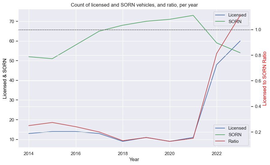
The numbers aren’t huge, but the number of Licensed has risen from ~10 to ~60 in only a couple of years, and SORN numbers have dropped by almost 20. Quite a comeback! I am curious where that other ~20 came from - perhaps forgotten in a barn (so neither Licensed nor SORN), or perhaps they came from the MISSINGs. You can also see where the LS ratio crossed the magical 1.0 line, the same time the Licensed and SORN lines crossed.
For whose who don’t know, this is the Sunbeam:
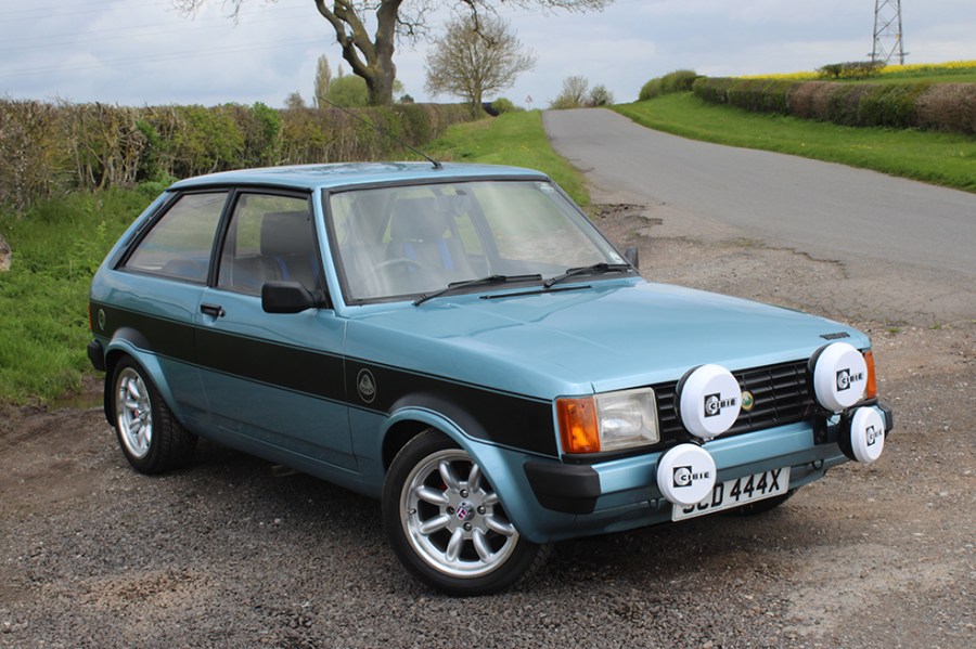
Image from https://classicsworld.co.uk/cars/talbot-sunbeam-lotus-road-test/
Different phoenixes
Of course, tweaks could be made to this search to get different results. For example:
- Adjusting the variables
- Add new checks, such as max number of SORN
- Searching all manufacture years (by removing
YearManufacturefrom the initial grouping) - Changing the cut-off year in the original data (for example, “modern classics”, vehicles pre 2010)
For example, by searching for cars with the LS ratio changeover and between 500 and 5000 Licensed in 2023 I found vehicles such as:
🐦🔥? LAND ROVER / LAND ROVER 88 / 88-4 CYL / 0
🐦🔥? TRIUMPH / TRIUMPH SPITFIRE / SPITFIRE / 0
🐦🔥? VOLKSWAGEN / VOLKSWAGEN 1300 / 1300 / 0
Searching for a 2023 LS ratio of over double the mean (vs 1x times in the original search), with over 500 Licensed vehicles in 2023, but at one time fewer than 500 included:
🐦🔥? MG / MG MGB / B / 1980
🐦🔥? MG / MG MGB / B GT / 1980
Vehicles where at one time the LS ratio was ≤0.5 (i.e. twice as many SORN as Licensed), but in 2023 the ratio is ≥2 (i.e. twice as many Licensed and SORN), with at least 20 currently Licensed (to avoid 0/1 → 1/0 etc), included a lot of classics, including:
🐦🔥? ALFA ROMEO / ALFA ROMEO 2000 / 2000 GT VELOCE / 1974
🐦🔥? JENSEN / JENSEN JENSEN-HEALEY / JENSEN-HEALEY / 1975
🐦🔥? LANCIA / LANCIA FULVIA / FULVIA / 1975
🐦🔥? PONTIAC / PONTIAC FIREBIRD / FIREBIRD / 1977
🐦🔥? RELIANT / RELIANT SCIMITAR / SCIMITAR GTC AUTO / 1980
You get the idea! As I’ve said, my script is available on GitHub (link at the top of this page), and the data is all on the DVLA website (again at the top of this page), so have a play yourself.
Some other classics
Given I had the data already processed, I also wanted to see the data for a few cars I know are classics. These didn’t show up in the searches for various reasons, mostly because the LS ratio never changed over - some have always had more Licensed than SORN; most have always had more SORN than Licensed (at least since 2014). A couple - the Supra, the Elise - did cross over, albeit in the wrong direction, so it would have failed the LS ratio > mean test. Regardless, some interesting trends:
Jaguar E-Type
Aston Martin DB5
Lotus Elise Series 1
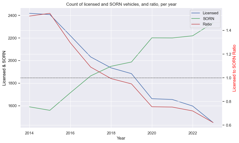
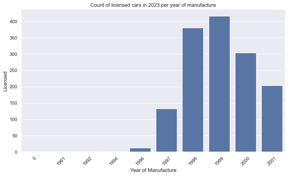
Peugeot 205 GTi
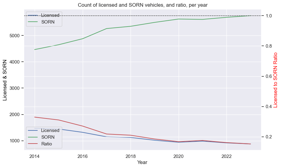
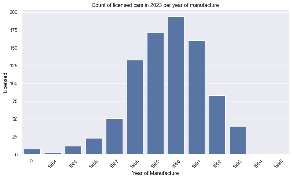
Ford Escort RS Cosworth
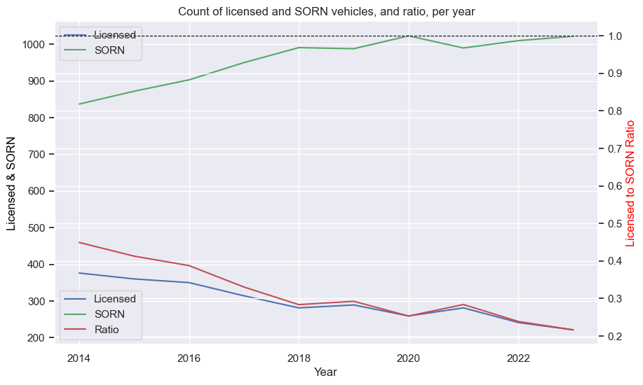
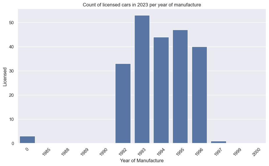
Mercedes-Benz 190E (Cosworth)
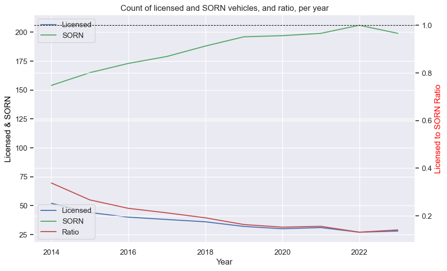
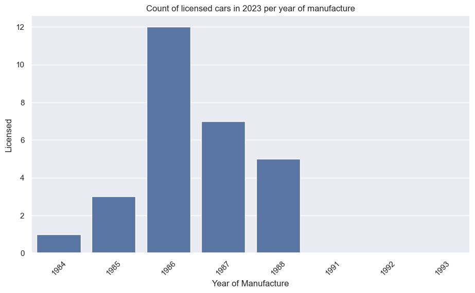
BMW E30 M3
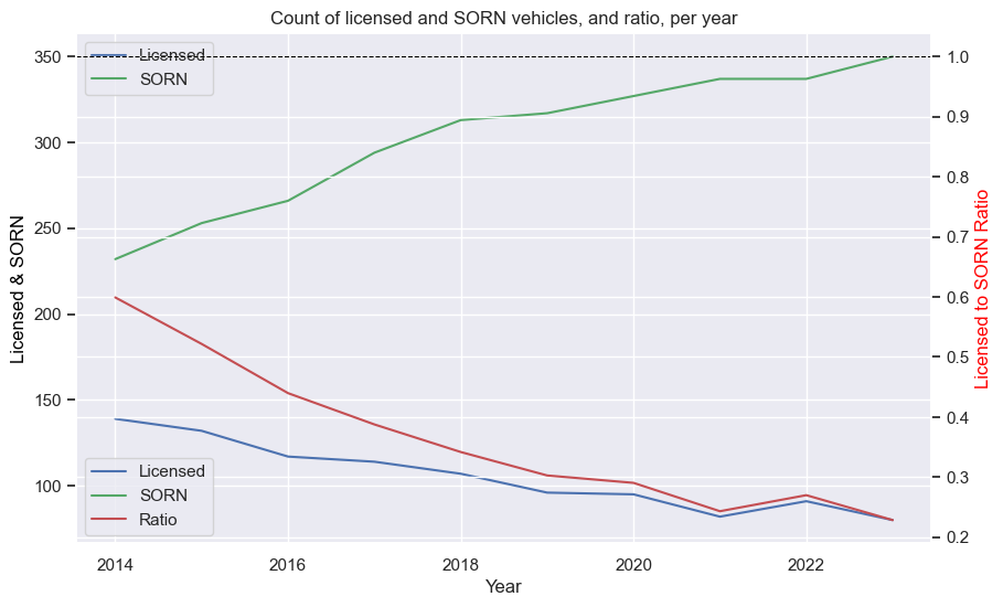
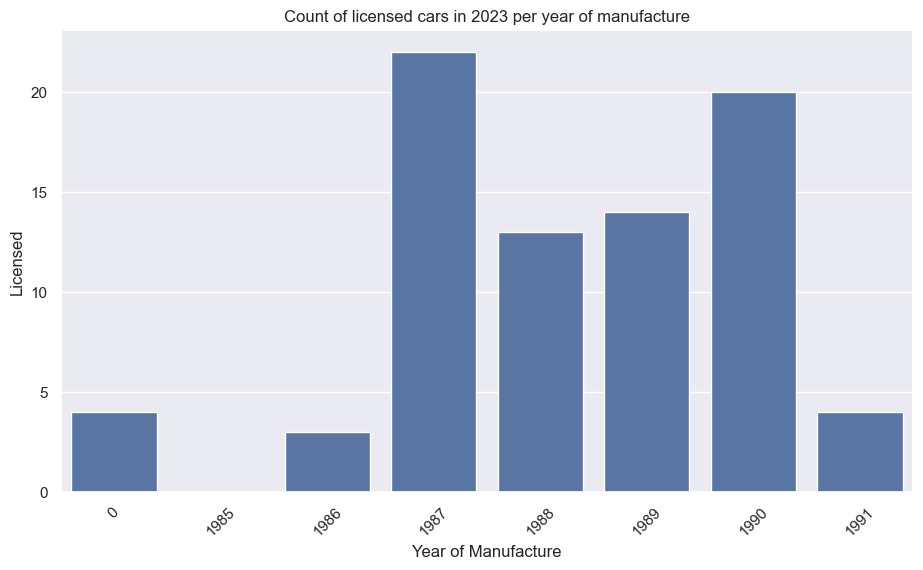
VW Golf GTI Mk1
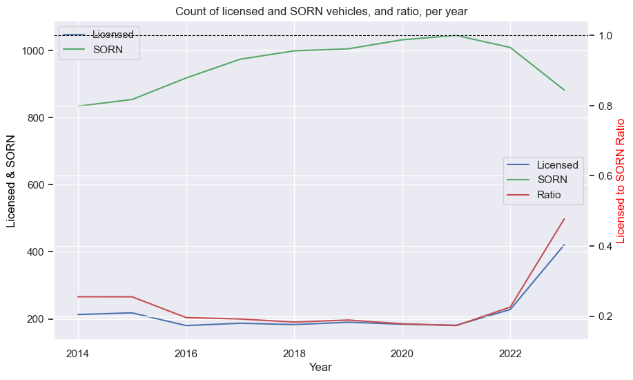
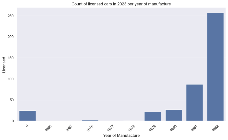
Porsche 911 (pre-1998)
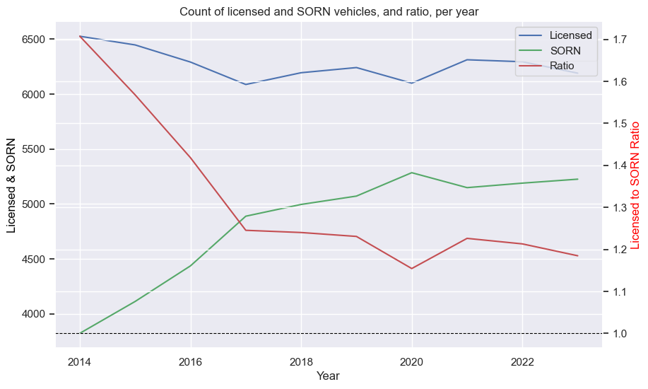
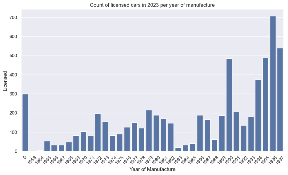
Toyota Supra
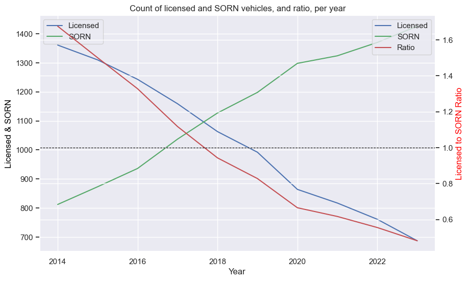
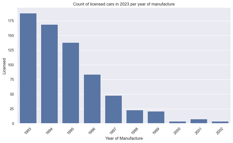
Mazda RX-7
Conclusion
This was fun! Using publicly-accessible data, transforming it, calculating new columns, plotting to observe trends, and then a custom search for vehicles fulfilling specific criteria.
Out of everything I’ve discovered, the old MGs and Triumphs really stood out. Several models have gone from more-SORN to more-Licensed, and they exist in high enough volumes that it’s actually feasible to buy one. Others - such as the Jensen or Lancia or Alfa - only had one or two for sale, or fewer, and they’re not cheap. Looking on Auto Trader, MGB GTs vary from £4k to £20, depending on condition; Triumph Stags are £10k to £30k. I’d be curious to see how the prices of these change over the coming years, especially with the move towards EVs - maybe there will be more demand for these small, retro British cars.
I went on to create a dashboard for this data using Power BI. You can see the post here: https://www.jamesgibbins.com/dvla-data-dashboard/
